Settings View Source Forecasting - fit to a known distribution

Fitting data to known distributions use is done using Chi2Fit.

This notebook describes how to use Chi2Fit for simple forecasting. This is illustrated for a team that takes up work items, exercises their expertise to complete the work. It shows one way for answering the questions: duration - how many iterations does it take to complete a certain number of items? completed items - how many items can be completed in a certain number of iterations? This note shows (a) what data to use, (b) how to read in the data, (c) assume a Poisson model for the data, and (d) estimate the average and variation to answer the above questions.

The advantages of this approach over directly fitting data (as shown in the notebook 'Forecasting-empirical-data') are:

• the Poisson distribution most often is a reasonable approximation for the team's throughtpu data,
• using the this assumption provides more strict bounds on the delivery rate parameter,
• the forecastting contains less variability

The disadvantages include:

• it assumes that the delivery rate of the team is constant over time,
• it assumes the Poisson model is reasonable enough model to describe the data.

table-of-contents

Table of contents

• Set-up
• Data and simulation set-up
• Preparation
• Forecasting using a Poisson distribution
• Rate error propagation: Total Monte Carlo
• References

set-up

Set-up

alias Chi2fit.Distribution, as: D
alias Chi2fit.Fit, as: F
alias Chi2fit.Matrix, as: M
alias Chi2fit.Utilities, as: U
alias Gnuplotlib, as: P
alias Exboost.Math

Exboost.Math

data-and-simulation-set-up

Data and simulation set-up

As an example consider the throughput of completed backlog items. At the end of a fixed time period we count the number of backlog items that a teram completes. Partially completed items are excluded from the count.

data = [3,3,4,4,7,5,1,11,5,6,3,6,6,5,4,10,4,5,8,2,4,12,5]

[3, 3, 4, 4, 7, 5, 1, 11, 5, 6, 3, 6, 6, 5, 4, 10, 4, 5, 8, 2, 4, 12, 5]

P.histogram(data,
    plottitle: "Throughput histogram",
    xlabel: "Throughput (items per 2 weeks)",
    ylabel: "Frequency",
    yrange: '[0:7]')
:"this is an inline image"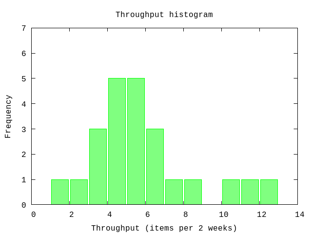

Other parameters that affect the forecasting are listed below. Please adjust to your needs.

# The size of the backlog, e.g. 100 backlog items
size = 100

# Number of iterations to use in the Monte Carlo
iterations = 1000

# The size of bins for grouping the data
binsize = 1

# Number of probes to use in the chi2 fit
probes = 10_000

# The range of the parameter to look for a (global) minimum
initial = {1,10}

{1, 10}

preparation

Preparation

Next, we convert the throughput data to a histogram. To this end we group the data in bins of size 1 starting at 0.

hdata = U.to_bins data, {binsize,0}

[{1, 0.043478260869565216, 0.0058447102657877, 0.13689038224309594}, {2, 0.08695652173913043, 0.02977628442357071, 0.1905937209791003}, {3, 0.21739130434782608, 0.1263699563343216, 0.33774551477037923}, {4, 0.43478260869565216, 0.3160946312914347, 0.5600249434832333}, {5, 0.6521739130434783, 0.5263221461493021, 0.7626298741894857}, {6, 0.782608695652174, 0.6622544852296207, 0.8736300436656784}, {7, 0.8260869565217391, 0.709703289667655, 0.9080712005244068}, {8, 0.8695652173913043, 0.7585954661422599, 0.9405937209791002}, {10, 0.9130434782608695, 0.8094062790208998, 0.9702237155764294}, {11, 0.9565217391304348, 0.8631096177569041, 0.9941552897342123}, {12, 1.0, 0.9225113769324543, 1.0}]

The data returned contains a list of tuples each describing a bin:

• the end-point of the bin,
• the proportional number of events for this bin (the total count is normalized to one),
• the lower value of the error bound,
• the upper value of the error bound.

As can be seen the sizes of the lower and upper bounds are different in value, i.e. they are asymmetrical. The contribution or weight to the likelihood function used in fitting known distributions will de different depending on whether the observed value if larger or smaller than the predicted value. This is specified by using the option :linear (see below). See [3] for details.

P.ecdf(hdata,
    plottitle: "Empirical CDF",
    xlabel: "Throughput (items per 2 weeks)",
    ylabel: "Probability",
    xrange: '[0:15]')
:"this is an inline image"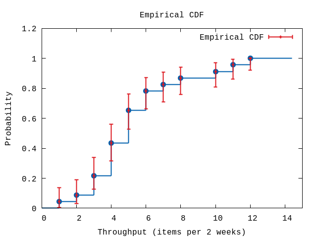

forecasting-using-a-poisson-distribution

Forecasting using a Poisson distribution

Instead of directly using the raw data captured one can also use a known probability distribution. The parameter of the distribution is matched to the data. After matching the parameter value one uses the known distribution to forecast.

Here, we will use the Poisson distribution [1]. This basically assumes that the data points are independent of each other.

The code below uses basic settings of the commands provided by Chi2Fit. More advanced options can be found at [2]. First a fixed number of random parameter values are tried to get a rough estimate. The option probes equals the number of tries. Furthermore, since we are fitting a probability distribution which has values on the interval [0,1] the errors are asymmetrical. This is specified by the option linear.

model = D.model "poisson"
options = [probes: probes, smoothing: false, model: :linear, saved?: true]
result = {_,parameters,_,saved} = F.chi2probe hdata, [initial], {Distribution.cdf(model), &F.nopenalties/2}, options
U.display result

Initial guess:
    chi2:       3.7680909998944285
    pars:       [5.467701988785316]
    ranges:     {[5.26279288835782, 5.687565561629632]}






:ok

The errors reported is the found range of parameter values where the corresponding chi2 values are within 1 of the found minimum value.

After roughly locating the minimum we do a more precise (and computationally more expensive) search for the minimum.

options = [{:probes,saved}|options]
result = {_,cov,parameters,_} = F.chi2fit hdata, {parameters, Distribution.cdf(model), &F.nopenalties/2}, 10, options
U.display(hdata,model,result,options)

Final:
    chi2:       3.7680887442307553
    Degrees of freedom: 10
    gradient:       [-4.284788519377549e-9]
    parameters:     [5.4680263772768605]
    errors:     [0.21599806132547897]
    ranges:
            chi2:       3.7680887442307553  -   4.752487946555217
            parameter:  5.26279288835782    -   5.687565561629632





:ok

For a (local) minimum the value of the gradient should be very close to zero.

P.ecdf(hdata,
    plottitle: "Fit of Poisson to CDF",
    xlabel: "Throughput (items per 2 weeks)",
    ylabel: "Probability",
    xrange: '[0:15]',
    title: "Poisson",
    func: & Distribution.cdf(model).(&1,parameters))
:"this is an inline image"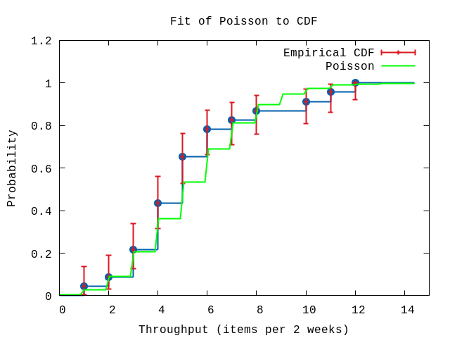

rate = hd(parameters)
pdf = fn x -> :math.pow(rate,x)*:math.exp(-rate)/Math.tgamma(x+1) end
P.pdf(data,
    plottitle: "Fit of PDF to Poisson",
    xlabel: "Throughput (items per 2 weeks)",
    ylabel: "Frequency",
    yrange: '[0:0.35]',
    pdf: pdf,
    title: "Poisson")
:"this is an inline image"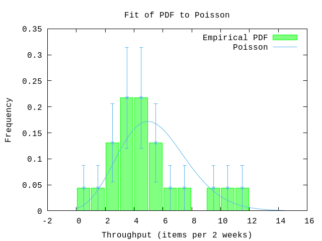

Again, using a Monte Carlo simulation we estimate the number of iterations and the range to expect.

{avg,sd,all} = U.mc(iterations, U.forecast_duration(fn -> Distribution.random(model).(parameters) end, size), collect_all?: true)
U.display {avg,sd,:+}

50%    => 19.0 units
84%    => 21.0 units
97.5%  => 23.0 units
99.85% => 25.0 units





:ok

P.histogram(all,
    plottitle: "Monte Carlo simulation for duration",
    xlabel: "Duration (number of iterations)",
    ylabel: "Frequency",
    xrange: '[0:30]')
:"this is an inline image"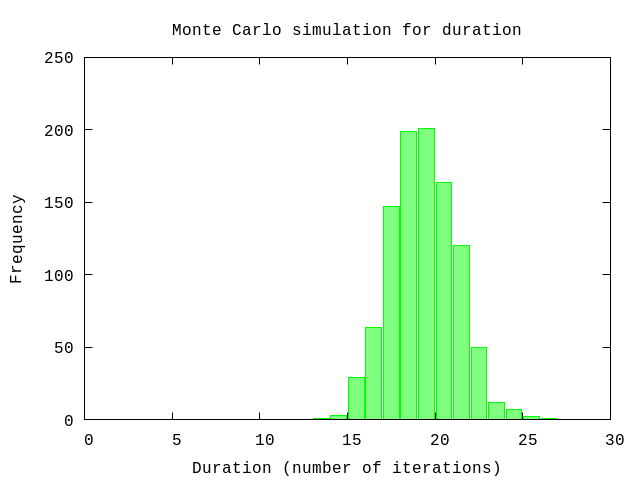

rate-error-propagation-total-monte-carlo

Rate error propagation: Total Monte Carlo

In the results of a Monte Carlo simulation the errors reported and the range of the number of iterations is the statistical error associated with the Monte Carlo simulation. It dopes not take into account the uncertainty of the parameter used in the fitted probability distribution function.

In Total Monte Carlo [4] multiple Monte Carlo simulations are done that correspond to the extreme values of the error bounds of the used parameters. The error results is of a different nature than the statistical error from the Monte Carlo simulation. These error reported separately.

# Pick up the error in the paramater value
param_errors = cov |> M.diagonal |> Enum.map(fn x->x|>abs|>:math.sqrt end)
[sd_rate] = param_errors

{avg_min,_} = U.mc(iterations, fn -> U.forecast(fn -> Distribution.random(model).([rate-sd_rate]) end, size) end)
{avg_max,_} = U.mc(iterations, fn -> U.forecast(fn -> Distribution.random(model).([rate+sd_rate]) end, size) end)

sd_min = avg - avg_max
sd_plus = avg_min - avg

IO.puts "Number of iterations to complete the backlog:"
IO.puts "#{Float.round(avg,1)} (+/- #{Float.round(sd,1)}) (-#{Float.round(sd_plus,1)} +#{Float.round(sd_min,1)})"

Number of iterations to complete the backlog:
18.8 (+/- 1.9) (-0.7 +0.8)





:ok

The first error is symmetric while the second error reported is asymmetric.

Combining the errors

We now have estimated two erros which have a different origin:

1. statistical error caused by the nature of the Poisson distribution as determined in Forecasting using a Poisson distribution, and
2. systematic error caused by the error in the deliveray rate in this section

Making the assumption that both are Gaussian - which is true for the systematic error but which is false for the systematic error - allows us to combine the two by quadratically addition.

sd_avg = (sd_plus + sd_min)/2
total = :math.sqrt sd*sd + sd_avg*sd_avg
U.display {avg,total,:+}

50%    => 19.0 units
84%    => 21.0 units
97.5%  => 23.0 units
99.85% => 25.0 units





:ok

references

References

[1] Poisson distribution, https://en.wikipedia.org/wiki/Poisson_distribution/<br> [2] Chi2Fit, Pieter Rijken, 2018, https://hex.pm/packages/chi2fit<br> [3] Asymmetric errors, Roger Barlow, Manchester University, UK and Stanford University, USA, PHYSTAT2003, SLAC, Stanford, California, September 8-11, 2003, https://www.slac.stanford.edu/econf/C030908/papers/WEMT002.pdf<br> [4] Efficient use of Monte Carlo: uncertainty propagation, D. Rochman et. al., Nuclear Science and Engineering, 2013, ftp://ftp.nrg.eu/pub/www/talys/bib_rochman/fastTMC.pdf