View Source Basic usage of the `Chi2fit` package

This notebook is based on Piotr Przetacznik's IElixir.

More information on Chi2fit can be found at:

What to find in this notebook?

Example notebooks
Elixir tutorial
Chi2fit Package
Available functions
Help
- Help on modules
- Help on functions
Additional packages
Usage
Special atoms
Inline images
Command history

example-notebooks
Example notebooks

A list of the notebooks that are available:

README.ipynb - this notebook ;-)
Forecasting-empirical-data.ipynb - directly using the empirical data to forecast
Forecasting-bootstrapping.ipynb - estimation of the error of the forecast because the data set is limited
Forecasting-fit-to-known-distribution.ipynb - description of the empirical data by a known probability distribution and use this to forecast
Forecasting-non-equilibrium.ipynb - analysis of changes in delivery rate to choose the most relevant and recent subsequence in the data set
Forecasting-multiplot.ipynb - demonstrates the use of multi plots
Forecasting-cycle-time.ipynb - illustrates analysis based on cycle time

The folder 'data' contains samples to use:

team.csv - data set containing less than 900 completion dates

A suggested reading order is shown below.

alias Graphvix.Graph, as: G
g = G.new node: [shape: "plaintext"]
{_, v1} = G.add_vertex g, "README.ipynb"
{_, v2} = G.add_vertex g, "Forecasting-empirical-data.ipynb"
{_, v3} = G.add_vertex g, "Forecasting-bootstrapping.ipynb"
{_, v4} = G.add_vertex g, "Forecasting-fit-to-known-distribution.ipynb"
{_, v5} = G.add_vertex g, "Forecasting-non-equilibrium.ipynb"
{_, v6} = G.add_vertex g, "Forecasting-multiplot.ipynb"
{_, v7} = G.add_vertex g, "Forecasting-cycle-time.ipynb"
G.add_edge g, v1, v2
G.add_edge g, v2, v3
G.add_edge g, v2, v4
G.add_edge g, v4, v5
G.add_edge g, v2, v6
G.add_edge g, v4, v7
:"do not show this result in output"

G.compile g, "/app/notebooks/images/readme", :png
{:"this is an inline image", src: "/app/notebooks/images/readme.png"}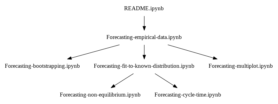

png

Several examples are included. Use the menu File -> open to explore which ones are available. Use thse to learn more about how to use Chi2fit or copy these as a basis for your own notes.

elixir-tutorial
Elixir tutorial

The notebooks are based on Jupyter and on the Elixir kernel. Commands and statements are entered using the language Elixir. There are many good tutorials on Elixir.

A good starting point is Elixir's home.

New to Elixir? An introduction to Elixir can be found here.

chi2fit-package
`Chi2fit` Package

The Chi2fit package consists of the (Elixir) modules:

And a module for drawing charts using Gnuplot:

Gnuplotlib

Finally, a contains the module Chi2fit.Cli for command line use outside of notebooks:

[Cli](* Cli

List of all available modules (see https://stackoverflow.com/questions/41733712/elixir-list-all-modules-in-namespace):

:application.load :chi2fit
with {:ok, list} <- :application.get_key(:chi2fit, :modules) do
  list |> Enum.filter(& &1 |> Module.split |> Enum.take(1) == ~w|Chi2fit|)
end

[Chi2fit.Cli, Chi2fit.Distribution, Chi2fit.Distribution.UnsupportedDistributionError, Chi2fit.FFT, Chi2fit.Fit, Chi2fit.Matrix, Chi2fit.Roots, Chi2fit.Utilities, Chi2fit.Utilities.UnknownSampleErrorAlgorithmError]

available-functions
Available functions

The functions provided by the modules are visible using the export function:

exports Chi2fit.Distribution

guess/1     guess/2     guess/3     model/1     model/2

help
Help

For all modules and function 'help' is available using the builtin command h.

Help on modules

h Chi2fit.Fit

[0m
[7m[33m                                  Chi2fit.Fit                                   [0m
[0m
Implements fitting a distribution function to sample data. It minimizes the
liklihood function.
[0m
[33m## Asymmetric Errors[0m
[0m
To handle asymmetric errors the module provides three ways of determining the
contribution to the likelihood function:
[0m
[36m    `simple` - value difference of the observable and model divided by the averaged error lower and upper bounds;
    `asimple` - value difference of the observable and model divided by the difference between upper/lower bound and the observed
      value depending on whether the model is larger or smaller than the observed value;
    `linear` - value difference of the observable and model divided by a linear tranformation (See below).[0m
[0m
[33m### 'linear': Linear transformation[0m
[0m
Linear transformation that:
[0m
[36m    - is continuous in u=0,
    - passes through the point sigma+ at u=1,
    - asymptotically reaches 1-y at u->infinity
    - pass through the point -sigma- at u=-1,
    - asymptotically reaches -y at u->-infinity[0m
[0m
[33m## References[0m
[0m
[1] See https://arxiv.org/pdf/physics/0401042v1.pdf
[0m

Help on functions

h Chi2fit.Distribution.model

[0m
[7m[33m                         def model(name, options \\ [])                         [0m
[0m
    [36m@spec[0m model(name :: String.t(), options :: Keyword.t()) :: any()

Returns the model for a name.
[0m
The kurtosis is the so-called 'excess kurtosis'.
[0m
Supported disributions:
[0m
[36m    "wald" - The Wald or Inverse Gauss distribution,
    "weibull" - The Weibull distribution,
    "exponential" - The exponential distribution,
    "poisson" - The Poisson distribution,
    "normal" - The normal or Gaussian distribution,
    "fechet" - The Fréchet distribution,
    "nakagami" - The Nakagami distribution,
    "sep" - The Skewed Exponential Power distribution (Azzalini),
    "erlang" - The Erlang distribution,
    "sep0" - The Skewed Exponential Power distribution (Azzalini) with location parameter set to zero (0).[0m
[0m
[33m## Options[0m
[0m
Available only for the SEP distribution, see 'sepCDF/5'.
[0m

additional-packages
Additional packages

The package Chi2fit is provided 'out-of-the-box' with this notebook. Additional packages can be installed from Hex.

IElixir provides a mechanism using Boyle.

Suppose we want to use the functions provided by Decimal.

Code.compiler_options [ignore_module_conflict: true]
Boyle.mk("decimal_env")
Boyle.list()

All dependencies up to date





{:ok, ["decimal_env"]}

Boyle.activate("decimal_env")
Boyle.install({:decimal, "~> 1.7"})

All dependencies up to date
Resolving Hex dependencies...
Dependency resolution completed:
New:
[32m  decimal 1.7.0[0m
* Getting decimal (Hex package)
==> decimal
Compiling 1 file (.ex)
Generated decimal app





:ok

sqrt2 = Decimal.sqrt("2")
Decimal.to_string(sqrt2)

"1.414213562373095048801688724"

ctxt = Decimal.get_context()
ctxt = %Decimal.Context{ctxt | precision: 50}
Decimal.set_context ctxt

:ok

sqrt2 = Decimal.sqrt("2")
Decimal.to_string(sqrt2)

"1.4142135623730950488016887242096980785696718753769"

Boyle.deactivate()

:ok

usage
Usage

Function need to be specified using the module name and function name, for example if we want the value of the Erlang CDF we use the function erlangCDF in the module Chi2fit.Distribution:

f = Chi2fit.Distribution.model "erlang", pars: [0.5,4.3]
Distribution.cdf(f).(0.1)

0.6462613084207343

We use an alias to have to type less:

alias Chi2fit.Distribution, as: D
f = D.model "erlang", pars: [0.5,4.3]
Distribution.cdf(f).(0.1)

0.6462613084207343

We can rid of the D. alltogether by using imports:

import Chi2fit.Distribution
f = model "erlang", pars: [0.5,4.3]
Distribution.cdf(f).(0.1)

0.6462613084207343

special-atoms
Special atoms

IElixir provides three atoms that are interpreted by IElixir.

What is an atom? In Elixir an atom ia a variable for which its value is its name. For example, the atmo :variable is an atom and has variable as value.

The 3 special atoms in IElixir are:

:"this is raw html" - the output result of the command is shown as is instead of an Elixir term
:"do not show this result in output" - the output of the statement is not shown in the output cell
:"this is an inline image" - used for displaying an image in the output cell (see below)

In addition to these atoms, the following tuple is interpreted:

{:"this is an inline image", src: path_to_image} - used for displaying an image in the output cell (see below)

These are used by returning either one of these as the result of a command.

inline-images
Inline images

The atom :"this is an inline image" indicates that the output of the cell is to be interpreted as a base64 encoded image.

An example based on Gnuplot is shown below.

Gnuplot.plot([
  ~w(set terminal pngcairo size 800,200)a,
  ~w(set output)a,
  [:plot, 'sin(x)', :title, "Sine Wave"]
])
Gnuplotlib.capture() |> Base.encode64 |> IO.write
:"this is an inline image"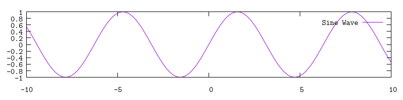

png

command-history
Command history

IElixir supports a simple command history. The results of the last command is stored in the variable ans.

:math.sqrt(2)

1.4142135623730951

ans

1.4142135623730951

The history of the results of previous commands can be accessed using the variable out.

i(out)

[33mTerm[0m
[22m  %{2 => [Chi2fit.Cli, Chi2fit.Distribution, Chi2fit.Distribution.UnsupportedDistributionError, Chi2fit.FFT, Chi2fit.Fit, Chi2fit.Matrix, Chi2fit.Roots, Chi2fit.Utilities, Chi2fit.Utilities.UnknownSampleErrorAlgorithmError], 6 => {:ok, ["decimal_env"]}, 7 => :ok, 8 => "1.414213562373095048801688724", 9 => :ok, 10 => "1.4142135623730950488016887242096980785696718753769", 11 => :ok, 12 => 0.6462613084207343, 13 => 0.6462613084207343, 14 => 0.6462613084207343, 16 => 1.4142135623730951, 17 => 1.4142135623730951}[0m
[33mData type[0m
[22m  Map[0m
[33mReference modules[0m
[22m  Map[0m
[33mImplemented protocols[0m
[22m  Ecto.DataType, Poison.Decoder, Poison.Encoder, IEx.Info, Collectable, Inspect, Enumerable, Timex.Protocol, CSV.Encode[0m

out[10]

"1.4142135623730950488016887242096980785696718753769"

← Previous Page API Reference

Next Page → Forecasting - based on empirical data

Settings View Source Basic usage of the Chi2fit package

example-notebooks Example notebooks

elixir-tutorial Elixir tutorial

chi2fit-package Chi2fit Package

available-functions Available functions

help Help