View Source Facets archiving
Mix.install(
  [{:lastfm_archive, path: "elixir/lastfm_archive"}, {:kino_explorer, "~> 0.1.10"}],
  config: [
    lastfm_archive: [
      data_dir: "./lastfm_data/",
      user: ""
    ]
  ]
)

alias Explorer.DataFrame
alias LastfmArchive.Livebook, as: LFM_LB

:ok
Introduction
lastfm_archive data stemmed from music tracks have been played over times and some, repeatedly. The data has multiple facets (aspects or dimensions). For example, what are the unique artists, albums or tracks within the listening history? When was a particular track played for the very first time or recently? Such faceted data may be derived from the scrobbles, typically from a column or columns subset of the archive.
Usually, facets data can be computated as required in runtime. For example, when a track was scrobbled, extra info can be used to check if it's new, popular or hasn't been played for awhile. This requires the entire listening history to be analysed in situ. For a larger dataset (e.g. 16-year listening history) this may be slow and computationally expensive.
This guide demonstrates how lastfm_archive can be used to derive the following types of archives which are essentially pre-created facet datasets. It also exemplifies the data usage in analytics and visualisation.
artistsalbumstracks
Prerequisite
- Setup, installation
- Creating a file archive containing scrobbles in raw JSON format fetched from Lastfm API
Creating a facet dataframe
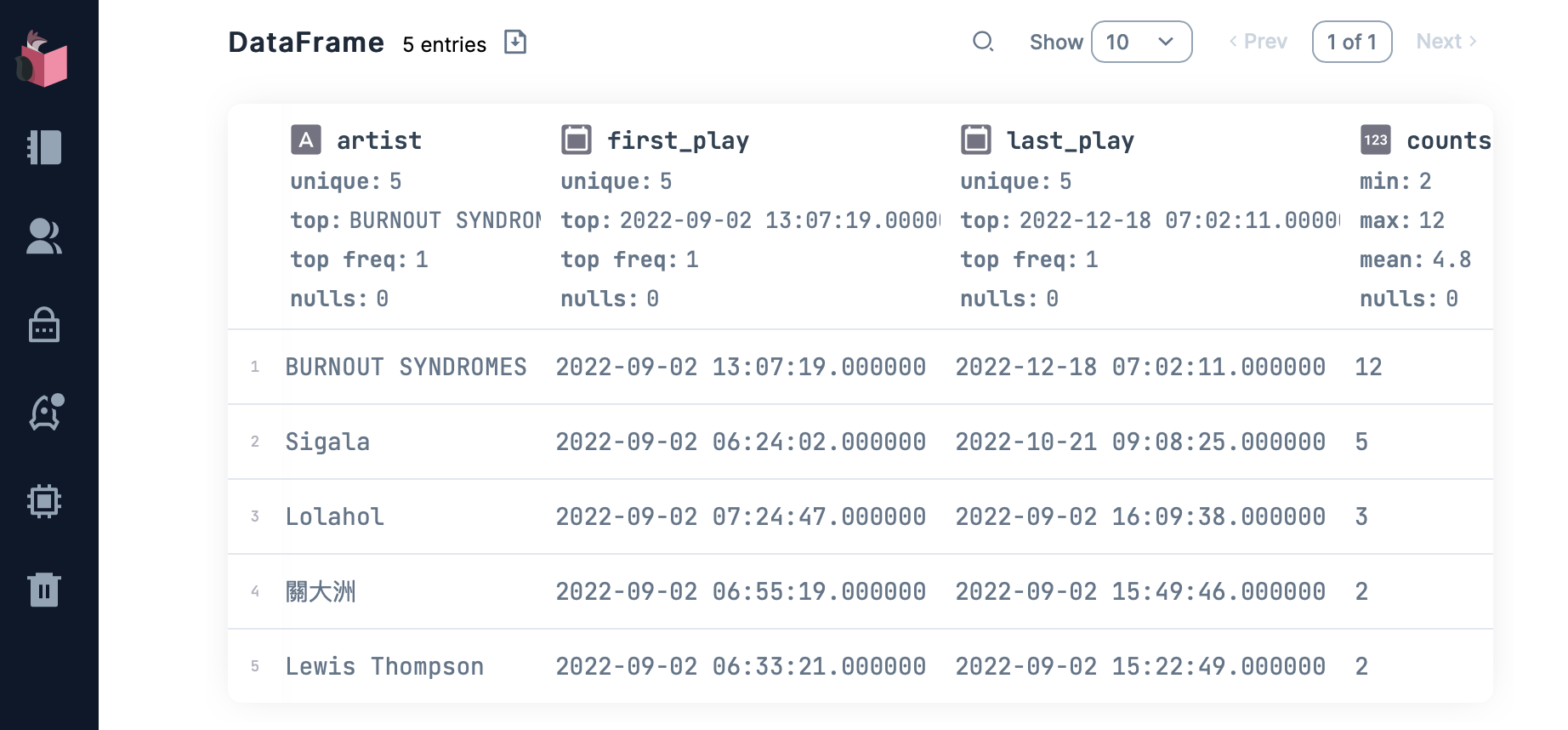
Using read/2 that returns a lazy dataframe of the entire listening history, a faceted dataframe can be created via the following pipeline. Aggregation is performed on a facet, e.g. the artist column, deriving all unique values and additional stats such as first_play - the earliest occurrence of an artist. Evaluate the code below to see a dataframe consisting all the artists to whom you have listened.
This pipeline is used in FacetsTransformer which is part of the lastfm_archive transform/2 function.
require DataFrame
{:ok, df} = LastfmArchive.default_user() |> LastfmArchive.read(format: :ipc_stream)

df
|> DataFrame.select([:artist, :datetime])
|> DataFrame.group_by([:artist])
|> DataFrame.summarise(counts: count(datetime), first_play: min(datetime))
|> DataFrame.arrange(desc: counts)
|> DataFrame.collect()
Facets archiving
lastfm_archive's transform function contains the above logic. It enables the creation of facet datasets using the following main options:
- facet:
:artists,:albumsor:tracks - format:
:ipc_stream,:ipc,:parquetor:csv
The archive is stored on a year-by-year basis so that subsequent data updates may be done without the need to re-genereate all previous data. Only the latest data (year) needs to be refreshed (via the year option).
LastfmArchive.default_user()
|> LastfmArchive.transform(facet: :tracks, format: :ipc_stream, overwrite: true)
Using faceted archive
The archives can be read and used in many ways. For example, the following identifies new artists played for the very first time on a particular date.
See a sample output.
require DataFrame
# change facet to `:albums` or `:tracks` to see other results
{:ok, df} = LastfmArchive.read(LastfmArchive.default_user(), facet: :artists, format: :ipc_stream)
# change these dates to ones that will yield results for your dataset
this_day_am = DateTime.new!(~D[2022-09-02], ~T[00:00:00], "Etc/UTC") |> DateTime.to_naive()
this_day_pm = DateTime.new!(~D[2022-09-02], ~T[23:59:59], "Etc/UTC") |> DateTime.to_naive()
df
|> DataFrame.filter(first_play > ^this_day_am and first_play < ^this_day_pm)
|> DataFrame.arrange(desc: counts)
|> DataFrame.head()
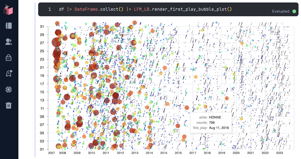
|> DataFrame.collect()You can also use the data in visualisation. For example, the following displays all artists and the time when their were discovered / first listened to, in a VegaLite bubble plot. Artists are represented by bubbles of different sizes and colours proportional to the overall total counts (popularity).
See a sample output generated from a Lastfm user's listening history.
The plot shows regular discovery of new artists. Artists discovered earlier are more "popular", i.e. more likelihood of repeats over time. You can see the source code of the plot here, look for the render_first_play_bubble_plot function.
df |> DataFrame.collect() |> LFM_LB.render_first_play_bubble_plot()Other transform options
The other transform/2 options may also be used for example, to overwrite existing year 2023 data (below) after new scrobbles have been synced from Lastfm. You can also regenerate the entire dataset with overwrite option without the year option.
LastfmArchive.default_user()
|> LastfmArchive.transform(facet: :artists, format: :ipc_stream, year: 2023, overwrite: true)