View Source Classifying horses and humans

Mix.install([
  {:axon, "~> 0.6.0"},
  {:nx, "~> 0.6.0"},
  {:exla, "~> 0.6.0"},
  {:stb_image, "~> 0.6.0"},
  {:req, "~> 0.4.5"},
  {:kino, "~> 0.11.0"}
])

Nx.global_default_backend(EXLA.Backend)
Nx.Defn.global_default_options(compiler: EXLA)

Introduction

In this notebook, we want to predict whether an image presents a horse or a human. To do this efficiently, we will build a Convolutional Neural Network (CNN) and compare the learning process with and without gradient centralization.

Loading the data

We will be using the Horses or Humans Dataset. The dataset is available as a ZIP with image files, we will download it using req. Conveniently, req will unzip the files for us, we just need to convert the filenames from strings.

%{body: files} =
  Req.get!("https://storage.googleapis.com/learning-datasets/horse-or-human.zip")

files = for {name, binary} <- files, do: {List.to_string(name), binary}

Note on batching

We need to know how many images to include in a batch. A batch is a group of images to load into the GPU at a time. If the batch size is too big for your GPU, it will run out of memory, in such case you can reduce the batch size. It is generally optimal to utilize almost all of the GPU memory during training. It will take more time to train with a lower batch size.

batch_size = 32
batches_per_epoch = div(length(files), batch_size)

A look at the data

We'll have a really quick look at our data. Let's see what we are dealing with:

{name, binary} = Enum.random(files)
Kino.Markdown.new(name) |> Kino.render()
Kino.Image.new(binary, :png)

Reevaluate the cell a couple times to view different images. Note that the file names are either horse[N]-[M].png or human[N]-[M].png, so we can derive the expected class from that.

While we are at it, look at this beautiful animation:

names_to_animate = ["horse01", "horse05", "human01", "human05"]

images_to_animate =
  for {name, binary} <- files, Enum.any?(names_to_animate, &String.contains?(name, &1)) do
    Kino.Image.new(binary, :png)
  end

Kino.animate(50, images_to_animate, fn
  _i, [image | images] -> {:cont, image, images}
  _i, [] -> :halt
end)

How many images are there?

length(files)

How many images will not be used for training? The remainder of the integer division will be ignored.

files
|> length()
|> rem(batch_size)

Data processing

First, we need to preprocess the data for our CNN. At the beginning of the process, we chunk images into batches. Then, we use the parse_file/1 function to load images and label them accurately. Finally, we "augment" the input, which means that we normalize data and flip the images along one of the axes. The last procedure helps a neural network to make predictions regardless of the orientation of the image.

defmodule HorsesHumans.DataProcessing do
  import Nx.Defn

  def data_stream(files, batch_size) do
    files
    |> Enum.shuffle()
    |> Stream.chunk_every(batch_size, batch_size, :discard)
    |> Task.async_stream(
      fn batch ->
        {images, labels} = batch |> Enum.map(&parse_file/1) |> Enum.unzip()
        {Nx.stack(images), Nx.stack(labels)}
      end,
      timeout: :infinity
    )
    |> Stream.map(fn {:ok, {images, labels}} -> {augment(images), labels} end)
    |> Stream.cycle()
  end

  defp parse_file({filename, binary}) do
    label =
      if String.starts_with?(filename, "horses/"),
        do: Nx.tensor([1, 0], type: {:u, 8}),
        else: Nx.tensor([0, 1], type: {:u, 8})

    image = binary |> StbImage.read_binary!() |> StbImage.to_nx()

    {image, label}
  end

  defnp augment(images) do
    # Normalize
    images = images / 255.0

    # Optional vertical/horizontal flip
    { u, _new_key } = Nx.Random.key(1987) |> Nx.Random.uniform()

    cond do
      u < 0.25 -> images
      u < 0.5 -> Nx.reverse(images, axes: [2])
      u < 0.75 -> Nx.reverse(images, axes: [3])
      true -> Nx.reverse(images, axes: [2, 3])
    end
  end
end

Building the model

The next step is creating our model. In this notebook, we choose the classic Convolutional Neural Network architecture. Let's dive in to the core components of a CNN.

Axon.conv/3 adds a convolutional layer, which is at the core of a CNN. A convolutional layer applies a filter function throughout the image, sliding a window with shape :kernel_size. As opposed to dense layers, a convolutional layer exploits weight sharing to better model data where locality matters. This feature is a natural fit for images.


Figure 1: A step-by-step visualization of a convolution layer for `kernel_size: {3, 3}`

Axon.max_pool/2 adds a downscaling operation that takes the maximum value from a subtensor according to :kernel_size.


Figure 2: Max pooling operation for `kernel_size: {2, 2}`

Axon.dropout/2 and Axon.spatial_dropout/2 add dropout layers which prevent a neural network from overfitting. Standard dropout drops a given rate of randomly chosen neurons during the training process. On the other hand, spatial dropout gets rid of whole feature maps. The graphical difference between dropout and spatial dropout is presented in a picture below.


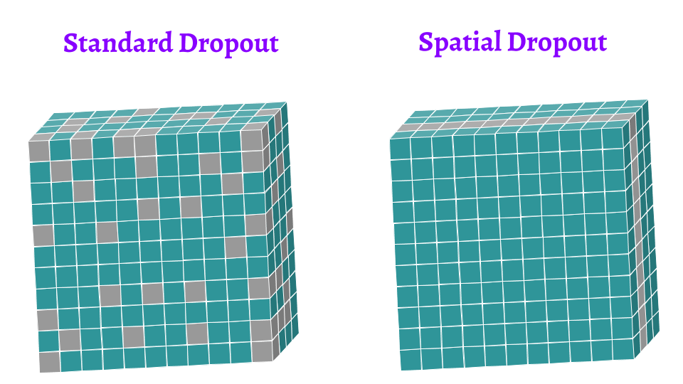Figure 3: The difference between standard dropout and spatial dropout

Knowing the relevant building blocks, let's build our network! It will have a convolutional part, composed of convolutional and pooling layers, this part should capture the spatial features of an image. Then at the end, we will add a dense layer with 512 neurons fed with all the spatial features, and a final two-neuron layer for as our classification output.

model =
  Axon.input("input", shape: {nil, 300, 300, 4})
  |> Axon.conv(16, kernel_size: {3, 3}, activation: :relu)
  |> Axon.max_pool(kernel_size: {2, 2})
  |> Axon.conv(32, kernel_size: {3, 3}, activation: :relu)
  |> Axon.spatial_dropout(rate: 0.5)
  |> Axon.max_pool(kernel_size: {2, 2})
  |> Axon.conv(64, kernel_size: {3, 3}, activation: :relu)
  |> Axon.spatial_dropout(rate: 0.5)
  |> Axon.max_pool(kernel_size: {2, 2})
  |> Axon.conv(64, kernel_size: {3, 3}, activation: :relu)
  |> Axon.max_pool(kernel_size: {2, 2})
  |> Axon.conv(64, kernel_size: {3, 3}, activation: :relu)
  |> Axon.max_pool(kernel_size: {2, 2})
  |> Axon.flatten()
  |> Axon.dropout(rate: 0.5)
  |> Axon.dense(512, activation: :relu)
  |> Axon.dense(2, activation: :softmax)

Training the model

It's time to train our model. We specify the loss, optimizer and choose accuracy as our metric. We also set log: 1 to frequently update the training progress. We manually specify the number of iterations, such that each epoch goes through all of the baches once.

data = HorsesHumans.DataProcessing.data_stream(files, batch_size)

optimizer = Polaris.Optimizers.adam(learning_rate: 1.0e-4)

params =
  model
  |> Axon.Loop.trainer(:categorical_cross_entropy, optimizer, log: 1)
  |> Axon.Loop.metric(:accuracy)
  |> Axon.Loop.run(data, %{}, epochs: 10, iterations: batches_per_epoch)

Extra: gradient centralization

We can improve the training by applying gradient centralization. It is a technique with a similar purpose to batch normalization. For each loss gradient, we subtract a mean value to have a gradient with mean equal to zero. This process prevents gradients from exploding.

centralized_optimizer = Polaris.Updates.compose(Polaris.Updates.centralize(), optimizer)

model
|> Axon.Loop.trainer(:categorical_cross_entropy, centralized_optimizer, log: 1)
|> Axon.Loop.metric(:accuracy)
|> Axon.Loop.run(data, %{}, epochs: 10, iterations: batches_per_epoch)

Inference

We can now use our trained model, let's try a couple examples.

{name, binary} = Enum.random(files)
Kino.Markdown.new(name) |> Kino.render()
Kino.Image.new(binary, :png) |> Kino.render()

input =
  binary
  |> StbImage.read_binary!()
  |> StbImage.to_nx()
  |> Nx.new_axis(0)
  |> Nx.divide(255.0)

Axon.predict(model, params, input)

Note: the model output refers to the probability that the image presents a horse and a human respectively.

You can find a validation set here, in case you want to experiment further!

← Previous Page Classifying handwritten digits

Next Page → Generating text with LSTM