View Source k-nearest neighbors (KNN)

Mix.install([
  {:scholar, "~> 0.3.0"},
  {:explorer, "~> 0.8.2", override: true},
  {:exla, "~> 0.7.2"},
  {:nx, "~> 0.7.2"},
  {:req, "~> 0.4.14"},
  {:kino_vega_lite, "~> 0.1.11"},
  {:kino, "~> 0.12.3"},
  {:kino_explorer, "~> 0.1.18"},
  {:tucan, "~> 0.3.1"}
])copy

Setup

We will use VegaLite, Explorer, and Scholar throughout this guide, so let's define some aliases:

require Explorer.DataFrame, as: DF
require Explorer.Series, as: S
require Explorer.Query, as: Q
alias Scholar.Neighbors.{KNNClassifier, KNNRegressor, BruteKNN}
alias Scholar.Metrics.{Classification, Regression}copy

And let's configure EXLA as our default backend (where our tensors are stored) and compiler (which compiles Scholar code) across the notebook and all branched sections:

Nx.global_default_backend(EXLA.Backend)
Nx.Defn.global_default_options(compiler: EXLA)
seed = 42
key = Nx.Random.key(42)copy

#Nx.Tensor<
  u32[2]
  EXLA.Backend<host:0, 0.3809581470.3464101900.76787>
  [0, 42]
>copy

Use cases

This notebook will cover the three primary applications of k-nearest Neighbors: classification, regression, and anomaly detection. Let's get started with a practical example. Imagine just moved to a new city, and you're here for the first time. Since you're an active person, you'd like to find a nearby gym with good facilities. What would you do? You'd probably start by searching for gyms on online maps. The search results might look something like this:

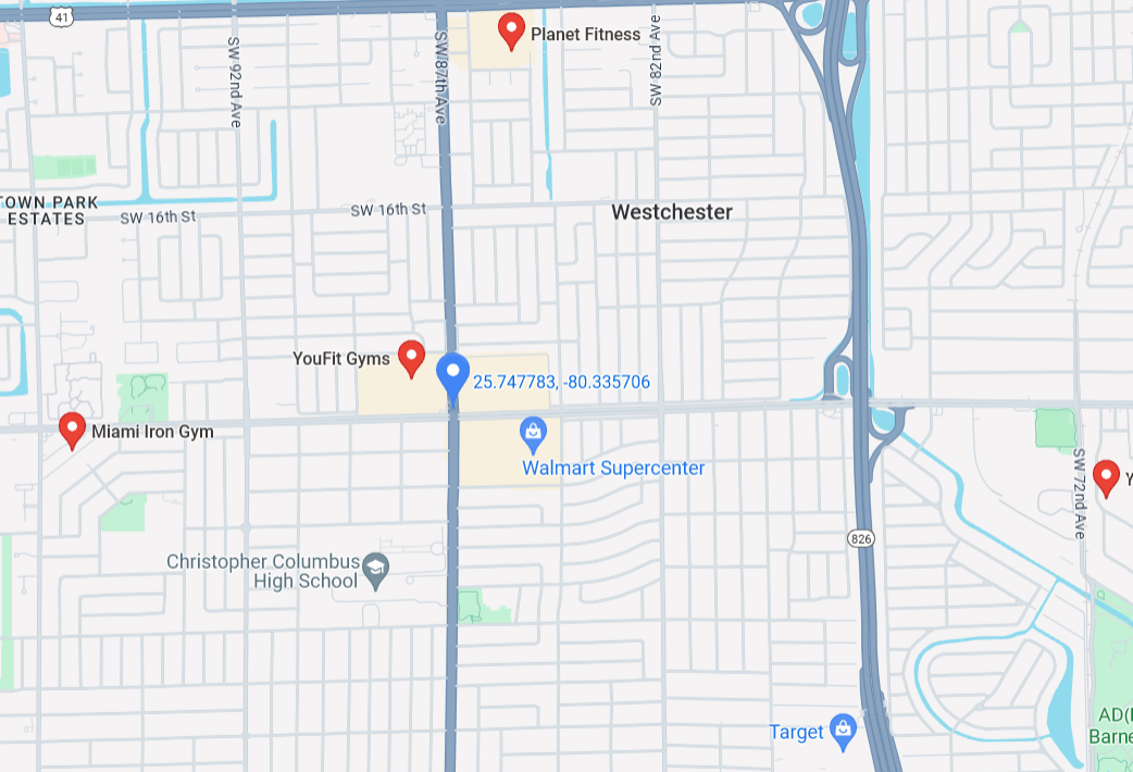
Now you can check out the gyms and eventually decide which one will be your regular spot. What did the search engine do? It calculated the nearest gyms (nearest neighbors) from your current location, which is the essence of finding nearest neighbors.

Now let's move to a more abstract example. You're listening to your favorite rock playlist and you think, "Yeah, these tracks are cool, but I've been listening to them on repeat. Maybe I should explore some new music." Searching for random songs might not be the most effective approach; you could end up with hip-hop or pop tracks, which you may not enjoy as much. However, it might also lead you to discover entirely new genres. A better approach could be to explore other rock playlists available online. While these playlists align with your preferred genre, they may not consider your unique tastes within rock music. Wouldn't it be great if there were a tool that could recommend new songs based on your previous playlists? Fortunately, such tools exist!

One type of recommendation system relies on collaborative filtering: it recommends songs based on what other users with similar musical tastes (aka its neighbours) listen to. Another approach is to treat songs as points and then compute the closest songs to your favorites. Part of the challenge in solving these problems is how to model users and songs as points in space however, once that is done, KNN algorithms play an essential role in understanding the relationships between them. So let's take a look at some concrete examples.

Classification

The process of classification using KNN is relatively straightforward. We start by working with a dataset where each sample is assigned a label. To predict the label of a new sample, we compute the distance between it and all the other samples in the dataset. Next, we select only the $k$ closest samples based on the distance metric, where $k$ is a user-defined parameter. We then examine the labels of these $k$ samples and choose the label that appears most frequently. This label is assigned as the predicted label for the new sample.

Let's first grasp how kNN works visually with a small example.

data =
  DF.new(
    x: [-1, 0.2, -0.5, -2.1, -2.3, -2.2, 0.1, 0.3, 0.4, 0.7, 1.3],
    y: [-0.1, 0.4, 0.5, 0.4, 1.1, -1.0, -0.1, 0.2, 1.5, 1.6, 0.9],
    label: [0, 0, 0, 0, 0, 0, 1, 1, 1, 1, 1]
  )

point_to_predict = DF.new(x: [0.0], y: [0.0])

k_eq_3 = DF.new(x: [0.45], y: [0.45], name: ["k = 3"])
k_eq_5 = DF.new(x: [0.72], y: [0.72], name: ["k = 5"])

radius = fn x, y -> :math.sqrt(x ** 2 + y ** 2) end

Tucan.layers([
  Tucan.scatter(data, "x", "y",
    point_size: 200,
    filled: true,
    shape_by: "label",
    color_by: "label"
  )
  |> Tucan.Scale.set_color_scheme(:plasma),
  Tucan.scatter(point_to_predict, "x", "y",
    point_size: 400,
    point_color: "green",
    point_shape: "triangle-up",
    filled: true
  ),
  Tucan.Geometry.circle({0, 0}, radius.(0.2, 0.4), line_color: "brown", stroke_width: 2),
  Tucan.Geometry.circle({0, 0}, radius.(-1, 0.1), line_color: "blue", stroke_width: 2),
  Tucan.annotate(Tucan.new(), 0.42, 0.42, "k = 3", color: "brown", size: 20),
  Tucan.annotate(Tucan.new(), 0.81, 0.81, "k = 5", color: "blue", size: 20)
])
|> Tucan.Scale.set_xy_domain(-2.4, 1.7)
|> Tucan.Grid.set_enabled(false)
|> Tucan.set_size(630, 630)
|> Tucan.set_title("Scatterplot showing KNN prediction process", offset: 20)copy

Note that the final prediction may vary depending on the value of $k$. For example, with $k = 3$, we would predict the green triangle as an orange square (1), whereas with $k = 5$, the purple circle (0) would be the final prediction.

Let's now test this using Scholar code. First, we will define our data.

x = Nx.stack(DF.discard(data, "label"), axis: 1)
labels = Nx.stack(DF.select(data, "label"), axis: 1) |> Nx.squeeze(axes: [1])
x_pred = Nx.stack(point_to_predict, axis: 1)copy

#Nx.Tensor<
  f64[1][2]
  EXLA.Backend<host:0, 0.3809581470.3464101900.76826>
  [
    [0.0, 0.0]
  ]
>copy

Let's now try with $k = 3$.

model = KNNClassifier.fit(x, labels, num_classes: 2, num_neighbors: 3, algorithm: :brute)
KNNClassifier.predict(model, x_pred)copy

#Nx.Tensor<
  s32[1]
  EXLA.Backend<host:0, 0.3809581470.3464101900.76922>
  [1]
>copy

And $k = 5$.

model = KNNClassifier.fit(x, labels, num_classes: 2, num_neighbors: 5, algorithm: :brute)
KNNClassifier.predict(model, x_pred)copy

#Nx.Tensor<
  s32[1]
  EXLA.Backend<host:0, 0.3809581470.3464101900.77007>
  [0]
>copy

As we can see, the predictions match our intuition from analyzing the plot.

Now, let's try KNN on a more complicated dataset: the Wine dataset. Our task will be to classify the quality of the wine. Before we load the dataset into Explorer.DataFrame for more efficient exploration, let's check some more detailed information about the dataset.

info =
  Req.get!(
    "https://archive.ics.uci.edu/ml/machine-learning-databases/wine-quality/winequality.names"
  ).body

Kino.Markdown.new(info)copy

data =
  Req.get!(
    "https://archive.ics.uci.edu/ml/machine-learning-databases/wine-quality/winequality-white.csv"
  ).body

df_data = DF.load_csv!(data, delimiter: ";", dtypes: %{"total sulfur dioxide": :float})
tensor_data = Nx.stack(df_data, axis: 1)
df_datacopy

#Explorer.DataFrame<
  Polars[4898 x 12]
  fixed acidity f64 [7.0, 6.3, 8.1, 7.2, 7.2, ...]
  volatile acidity f64 [0.27, 0.3, 0.28, 0.23, 0.23, ...]
  citric acid f64 [0.36, 0.34, 0.4, 0.32, 0.32, ...]
  residual sugar f64 [20.7, 1.6, 6.9, 8.5, 8.5, ...]
  chlorides f64 [0.045, 0.049, 0.05, 0.058, 0.058, ...]
  free sulfur dioxide f64 [45.0, 14.0, 30.0, 47.0, 47.0, ...]
  total sulfur dioxide f64 [170.0, 132.0, 97.0, 186.0, 186.0, ...]
  density f64 [1.001, 0.994, 0.9951, 0.9956, 0.9956, ...]
  pH f64 [3.0, 3.3, 3.26, 3.19, 3.19, ...]
  sulphates f64 [0.45, 0.49, 0.44, 0.4, 0.4, ...]
  alcohol f64 [8.8, 9.5, 10.1, 9.9, 9.9, ...]
  quality s64 [6, 6, 6, 6, 6, ...]
>copy

As we can see, there are no null values in the dataset. Now, let's check the size of the dataset.

DF.shape(df_data)copy

{4898, 12}copy

Let's check some statistical properties of the dataset. We will start with skewness, which measures the asymmetry of the probability distribution of a random variable about its mean. To better understand this concept, please take a look at the picture below.

Figure 1: A general relationship of mean and median under differently skewed unimodal distribution

Now, let's check the skewness of our dataset using Scholar.Stats.skew/1 function.

Scholar.Stats.skew(tensor_data)copy

#Nx.Tensor<
  f64[12]
  EXLA.Backend<host:0, 0.3809581470.3464101900.77136>
  [0.6475530855160632, 1.5764965159574844, 1.2815277799152376, 1.0767638711454446, 5.0217921696710315, 1.4063140718346212, 0.3905901775815236, 0.9774735389046988, 0.45764233925379794, 0.9768943947733456, 0.4871927332763434, 0.15574868141362447]
>copy

As we can see, all features have positive skewness, which means that their distributions are more similar to the left plot in the picture above.

Moving on to another statistical function, let's discuss kurtosis. Kurtosis measures how much data is located in the tails of distributions. If the kurtosis is greater than 0, the distribution is said to be "platykurtic", indicating that it has more extreme values than a univariate normal distribution. Similarly, a "leptokurtic" distribution has positive kurtosis and less extreme values, while a "mesokurtic" distribution has the same kurtosis as a normal distribution. Let's check the kurtosis of our dataset.

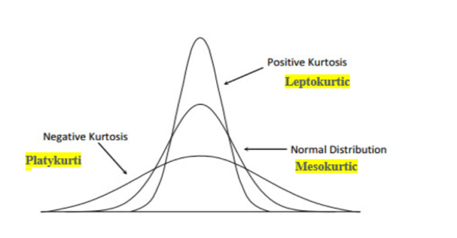Figure 2: Plot showing Platykurtic, Mesokurtic and Leptokurtic distributions

Scholar.Stats.kurtosis(tensor_data)copy

#Nx.Tensor<
  f64[12]
  EXLA.Backend<host:0, 0.3809581470.3464101900.77187>
  [2.168736944824719, 5.08520490451785, 6.167374226819426, 3.4650542966046363, 37.52503905008619, 11.453415905047144, 0.5700448984658735, 9.78258726703508, 0.5290085383907339, 1.5880812942840778, -0.6989373013774784, 0.21508011570192975]
>copy

Almost all features have positive kurtosis (they are leptokurtic). alcohol has negative excess kurtosis, which means it is platykurtic. Below there is Kernel Density Estimate (KDE) to check how exactly this tail look like.

# Increase the sample size (or use 1.0 to plot all data)
sample = DF.sample(df_data, 0.5, seed: seed)

Tucan.hconcat([
  Tucan.density(sample, "alcohol", only: ["alcohol"], fill_color: "lightblue")
  |> Tucan.Axes.set_x_title("% of alcohol")
  |> Tucan.set_size(350, 300)
  |> Tucan.set_title("KDE plot of alcohol feature", offset: 20),
  Tucan.density(sample, "pH", only: ["pH"], fill_color: "lightgreen")
  |> Tucan.set_size(350, 300)
  |> Tucan.set_title("KDE plot of pH feature", offset: 20)
])
|> Tucan.set_title("KDE plots of Features", anchor: :middle, offset: 20)copy

The previous analysis indicates that the alcohol feature has more extreme values than pH. Now, we will create a correlation heatmap to investigate the relationships between the features in the dataset.

correlation = Scholar.Stats.correlation_matrix(tensor_data, ddof: 1)copy

#Nx.Tensor<
  f64[12][12]
  EXLA.Backend<host:0, 0.3809581470.3464101900.77237>
  [
    [1.000204206657137, -0.022701925084394028, 0.28923975031725996, 0.08903887998201279, 0.02309035789846668, -0.04940594604443256, 0.09108835320911231, 0.26538519619855744, -0.42594525408939937, -0.017146485732801857, -0.12090580792461156, -0.1136860414197186],
    [-0.022701925084394028, 1.0002042066571377, -0.14950233378736394, 0.06429918773242695, 0.070525970411686, -0.0970317497617824, 0.08927873114082308, 0.027119382290178354, -0.03192188560415534, -0.035735442831260074, 0.06773177122976645, -0.19476273264768545],
    [0.28923975031725996, -0.14950233378736394, 1.000204206657138, 0.09423086293135367, 0.11438780236851878, 0.09409643220951228, 0.12115553337968561, 0.14953309999019224, -0.16378164987548596, 0.062343668678184735, -0.07574419436799362, -0.009210971441640103],
    [0.08903887998201279, 0.06429918773242695, 0.09423086293135367, 1.0002042066571373, 0.0887026459138499, 0.29915943156848096, 0.40152128773970025, 0.8391377774397895, -0.1941730973339338, -0.026669810894874028, -0.4507232439271815, -0.09759675473273582],
    [0.02309035789846668, 0.070525970411686, ...],
    ...
  ]
>copy

{corr_size, _} = Nx.shape(correlation)
correlation_list = Nx.to_flat_list(correlation)
column_names = DF.names(df_data)

corr_to_plot =
  DF.new(
    x: List.flatten(List.duplicate(column_names, corr_size)),
    y: List.flatten(for name <- column_names, do: List.duplicate(name, corr_size)),
    corr_val: Enum.map(correlation_list, fn x -> Float.round(x, 2) end)
  )

Tucan.heatmap(corr_to_plot, "x", "y", "corr_val", annotate: true, text_color: [{nil, 0, "white"}])
|> Tucan.Scale.set_color_scheme(:inferno)
|> Tucan.Axes.set_title(:color, "Correlation")
|> Tucan.set_size(630, 630)
|> Tucan.set_title("Correlation Matrix for California Housing", offset: 20)copy

We can observe from the correlation heatmap that there is no strong correlation between the quality of wine and any single feature. However, we can see that there are two strong correlations: density is proportional to the amount of residual sugar and inversely proportional to the amount of alcohol.

Given that citric acid, free sulfur dioxide, and sulphates are not strongly correlated with the quality of wine or any other features, we can drop them from the dataset to simplify our analysis.

Before dropping the features, it is important to consider their potential impact on the final prediction. Even if they are not strongly correlated with the target variable (quality), they may still provide useful information for the KNN algorithm. It is recommended to experiment with different feature subsets to find the optimal combination for the given task. You can try running the notebook again without dropping these features.

tensor_data =
  DF.discard(df_data, ["citric acid", "free sulfur dioxide", "sulphates"]) |> Nx.stack(axis: 1)copy

#Nx.Tensor<
  f64[4898][9]
  EXLA.Backend<host:0, 0.3809581470.3464101900.77289>
  [
    [7.0, 0.27, 20.7, 0.045, 170.0, 1.001, 3.0, 8.8, 6.0],
    [6.3, 0.3, 1.6, 0.049, 132.0, 0.994, 3.3, 9.5, 6.0],
    [8.1, 0.28, 6.9, 0.05, 97.0, 0.9951, 3.26, 10.1, 6.0],
    [7.2, 0.23, 8.5, 0.058, 186.0, 0.9956, 3.19, 9.9, 6.0],
    [7.2, 0.23, 8.5, 0.058, 186.0, 0.9956, 3.19, 9.9, 6.0],
    [8.1, 0.28, 6.9, 0.05, 97.0, ...],
    ...
  ]
>copy

The next step will be splitting the dataset into features and labels. To make the classification task easier, we will convert the labels into three categories: "poor," "medium," and "excellent". Additionally, we will normalize the features using the standard scaler.

x = tensor_data[[.., 0..-2//1]]
y = tensor_data[[.., -1]]

# convert quality into labels quality: (0, 4) poor => 0, (5, 6) medium => 1, (7, 10) excelent => 2

poor_and_better_mask = Nx.greater(y, 4)
medium_and_better_mask = Nx.greater(y, 6)

y = Nx.select(poor_and_better_mask, Nx.select(medium_and_better_mask, 2, 1), 0)
x = Scholar.Preprocessing.standard_scale(x)

{x, y}copy

{#Nx.Tensor<
   f64[4898][8]
   EXLA.Backend<host:0, 0.3809581470.3464101900.77349>
   [
     [-0.29385297541380284, -0.4368649169854585, -0.0027291121847267076, -0.44164614831586296, 3.1698834995014824, -0.4213312276408997, -0.37885264350988346, -0.2556031247705665],
     [-0.30872791733061694, -0.43622741947473787, -0.40860252734351166, -0.4415611486477669, 2.3623866525887167, -0.4214799770600679, -0.3724776684026774, -0.24072818285375244],
     [-0.27047806668738067, -0.43665241781521824, -0.29597796711620483, -0.4415398987307429, 1.6186395567480112, -0.42145660215134145, -0.37332766508363824, -0.22797823263934036],
     [-0.2896029920089988, -0.4377149136664193, -0.2619780998777726, -0.44136989939455074, 3.509882171885805, -0.42144597719282945, -0.3748151592753196, -0.23222821604414437],
     [-0.2896029920089988, -0.4377149136664193, -0.2619780998777726, -0.44136989939455074, 3.509882171885805, -0.42144597719282945, -0.3748151592753196, -0.23222821604414437],
     [-0.27047806668738067, -0.43665241781521824, -0.29597796711620483, -0.4415398987307429, 1.6186395567480112, -0.42145660215134145, -0.37332766508363824, -0.22797823263934036],
     [-0.310852909033019, ...],
     ...
   ]
 >,
 #Nx.Tensor<
   s32[4898]
   EXLA.Backend<host:0, 0.3809581470.3464101900.77326>
   [1, 1, 1, 1, 1, 1, 1, 1, 1, 1, 1, 1, 1, 2, 1, 2, 1, 2, 1, 1, 2, 2, 2, 1, 1, 1, 1, 1, 1, 2, 1, 1, 1, 1, 1, 1, 1, 1, 1, 1, 1, 1, 1, 1, 1, 2, 0, 1, ...]
 >}copy

After performing EDA on our wine dataset, we can now train our KNN model and make predictions. However, the question arises as to what value of neighbors should we choose for the KNN model. To answer this question, we will use K-Fold Cross-Validation (specifically, Nested Cross-Validation). K-Fold is a procedure performed on the training dataset where we split the data into k smaller subsets (folds). For each tested parameter value, we run k separate trainings and testings, where one fold is the validation (test) dataset, and the other k-1 folds are the training dataset. To make this process clear, there is a GIF below that explains it visually.

Figure 3: Illustration of KFold Cross-Validation when n = 12 observations and k = 3. After data is shuffled, a total of 3 models will be trained and tested.

defmodule Comb do
  def combinations([]), do: [[]]

  def combinations([{name, values} | opts]) do
    for subcombination <- combinations(opts), value <- values do
      [{name, value} | subcombination]
    end
  end
end

Comb.combinations(task: [:classification], num_classes: [3], num_neighbors: Enum.to_list(1..30))copy

[
  [task: :classification, num_classes: 3, num_neighbors: 1],
  [task: :classification, num_classes: 3, num_neighbors: 2],
  [task: :classification, num_classes: 3, num_neighbors: 3],
  [task: :classification, num_classes: 3, num_neighbors: 4],
  [task: :classification, num_classes: 3, num_neighbors: 5],
  [task: :classification, num_classes: 3, num_neighbors: 6],
  [task: :classification, num_classes: 3, num_neighbors: 7],
  [task: :classification, num_classes: 3, num_neighbors: 8],
  [task: :classification, num_classes: 3, num_neighbors: 9],
  [task: :classification, num_classes: 3, num_neighbors: 10],
  [task: :classification, num_classes: 3, num_neighbors: 11],
  [task: :classification, num_classes: 3, num_neighbors: 12],
  [task: :classification, num_classes: 3, num_neighbors: 13],
  [task: :classification, num_classes: 3, num_neighbors: 14],
  [task: :classification, num_classes: 3, num_neighbors: 15],
  [task: :classification, num_classes: 3, num_neighbors: 16],
  [task: :classification, num_classes: 3, num_neighbors: 17],
  [task: :classification, num_classes: 3, num_neighbors: 18],
  [task: :classification, num_classes: 3, num_neighbors: 19],
  [task: :classification, num_classes: 3, num_neighbors: 20],
  [task: :classification, num_classes: 3, num_neighbors: 21],
  [task: :classification, num_classes: 3, num_neighbors: 22],
  [task: :classification, num_classes: 3, num_neighbors: 23],
  [task: :classification, num_classes: 3, num_neighbors: 24],
  [task: :classification, num_classes: 3, num_neighbors: 25],
  [task: :classification, num_classes: 3, num_neighbors: 26],
  [task: :classification, num_classes: 3, num_neighbors: 27],
  [task: :classification, num_classes: 3, num_neighbors: 28],
  [task: :classification, num_classes: 3, num_neighbors: 29],
  [task: :classification, num_classes: 3, num_neighbors: 30]
]copy

The code implementing KFold cross-validation is located at the beginning of the notebook.

min_num_neighbors = 1
param_space_size = 30

# K in KFold
k = 10
train_size = 4000

{indices, _new_key} = Nx.Random.shuffle(key, Nx.iota(Nx.shape(y)))
x = Nx.take(x, indices)
y = Nx.take(y, indices)
{train_data, test_data} = Nx.split(x, train_size)
{train_labels, test_labels} = Nx.split(y, train_size)

folding_fun = fn x -> Scholar.ModelSelection.k_fold_split(x, k) end

scoring_fun = fn x, y, opts ->
  {x_train, x_test} = x
  {y_train, y_test} = y

  model =
    KNNClassifier.fit(x_train, y_train,
      num_classes: opts[:num_classes],
      num_neighbors: opts[:num_neighbors],
      algorithm: :brute
    )

  prediction = KNNClassifier.predict(model, x_test)

  accuracy = Classification.accuracy(y_test, prediction)
  [accuracy]
end

res =
  Scholar.ModelSelection.grid_search(train_data, train_labels, folding_fun, scoring_fun,
    num_classes: [3],
    num_neighbors: Enum.to_list(min_num_neighbors..param_space_size)
  )

res = for(sub_res <- res, do: sub_res[:score]) |> Nx.concatenate() |> Nx.as_type(:f64)

results =
  DF.new(accuracy: res, num_neighbors: Nx.add(Nx.iota({param_space_size}), min_num_neighbors))copy

#Explorer.DataFrame<
  Polars[30 x 2]
  accuracy f64 [0.7682499885559082, 0.734250009059906, 0.7425000071525574, 0.7512499690055847, 0.7512499690055847, ...]
  num_neighbors s64 [1, 2, 3, 4, 5, ...]
>copy

To potentially improve our KNN model's performance, we can try setting the weights parameter to :distance and use weighted version of grid search. Next, we can visualize the results of KFold using a plot.

Tucan.lineplot(results, "num_neighbors", "accuracy",
  line_color: "gray",
  points: true,
  stroke_dash: [5, 5]
)
|> Tucan.Scale.set_x_domain(1, 31)
|> Tucan.Scale.set_y_domain(0.7, 0.85)
|> Tucan.set_size(630, 630)
|> Tucan.set_title("Accuracy vs Number of Neighbors", offset: 20)copy

best_neighbors = Nx.add(Nx.argmax(res), min_num_neighbors) |> Nx.to_number()copy

1copy

Ok, let's test our best model on test data.

best_model =
  KNNClassifier.fit(train_data, train_labels,
    num_neighbors: best_neighbors,
    num_classes: 3,
    algorithm: :brute
  )

final_prediction = KNNClassifier.predict(best_model, test_data)
Classification.accuracy(test_labels, final_prediction)copy

#Nx.Tensor<
  f32
  EXLA.Backend<host:0, 0.3809581470.3464101899.76876>
  0.7672605514526367
>copy

Pretty well, now let's move on to a regression task using KNN.

Regression

KNNs can also be used in regression tasks. We will explore this on a dataset about Airfoil Self-Noise. Here's a brief description of the dataset:

Data Set Information:

The NASA data set comprises different size NACA 0012 airfoils at various wind tunnel speeds and angles of attack. The span of the airfoil and the observer position were the same in all of the experiments.

Attribute Information:

This problem has the following inputs:

1. Frequency, in Hertzs.
2. Angle of attack, in degrees.
3. Chord length, in meters.
4. Free-stream velocity, in meters per second.
5. Suction side displacement thickness, in meters.

The only output is:

1. Scaled sound pressure level, in decibels.

Dua, D. and Graff, C. (2019). UCI Machine Learning Repository [http://archive.ics.uci.edu/ml]. Irvine, CA: University of California, School of Information and Computer Science.

dataset =
  Req.get!(
    "https://archive.ics.uci.edu/ml/machine-learning-databases/00291/airfoil_self_noise.dat"
  ).body

column_names = [
  "frequency",
  "angle_of_attack",
  "chord_length",
  "free_stream_velocity",
  "suction_side_displacement_thickness",
  "scaled_sound_pressure_level"
]

dataset_df = DF.load_csv!(dataset, header: false, delimiter: "\t") |> DF.rename(column_names)
labels = DF.select(dataset_df, "scaled_sound_pressure_level")
data = DF.discard(dataset_df, "scaled_sound_pressure_level")copy

#Explorer.DataFrame<
  Polars[1503 x 5]
  frequency s64 [800, 1000, 1250, 1600, 2000, ...]
  angle_of_attack f64 [0.0, 0.0, 0.0, 0.0, 0.0, ...]
  chord_length f64 [0.3048, 0.3048, 0.3048, 0.3048, 0.3048, ...]
  free_stream_velocity f64 [71.3, 71.3, 71.3, 71.3, 71.3, ...]
  suction_side_displacement_thickness f64 [0.00266337, 0.00266337, 0.00266337, 0.00266337, 0.00266337, ...]
>copy

Below are the KDE plots of the dataset's features. We will analyze them in the next step.

Tucan.concat(
  [
    Tucan.density(data, "frequency", fill_color: "lightblue", only: ["frequency"])
    |> Tucan.Axes.set_x_title("Frequency (Hz)")
    |> Tucan.set_size(350, 300)
    |> Tucan.set_title("KDE plot of Frequency feature", offset: 20),
    Tucan.density(data, "free_stream_velocity",
      fill_color: "purple",
      only: ["free_stream_velocity"]
    )
    |> Tucan.Axes.set_x_title("Angle of attack")
    |> Tucan.set_size(350, 300)
    |> Tucan.set_title("KDE plot of Angle of Attack feature", offset: 20),
    Tucan.density(data, "angle_of_attack", fill_color: "lightgreen", only: ["angle_of_attack"])
    |> Tucan.Axes.set_x_title("Angle of attack")
    |> Tucan.set_size(350, 300)
    |> Tucan.set_title("KDE plot of Angle of Attack feature", offset: 20),
    Tucan.density(data, "suction_side_displacement_thickness",
      fill_color: "red",
      only: ["suction_side_displacement_thickness"]
    )
    |> Tucan.Axes.set_x_title("Suction Side Displacement Thickness")
    |> Tucan.set_size(350, 300)
    |> Tucan.set_title("KDE plot of Suction Side Displacement\nThickness feature", offset: 20)
  ],
  columns: 2
)
|> Tucan.set_title("KDE plots of Features", anchor: :middle, offset: 20)copy

The Suction Side Displacement Thickness and Frequency features have asymmetric distributions with many observations having small values. To make these distributions less skewed, we will use the logarithms of these two features.

data =
  DF.mutate(data,
    frequency_log: log(frequency),
    suction_side_displacement_thickness_log: log(suction_side_displacement_thickness)
  )

data = DF.discard(data, ["frequency", "suction_side_displacement_thickness"])copy

#Explorer.DataFrame<
  Polars[1503 x 5]
  angle_of_attack f64 [0.0, 0.0, 0.0, 0.0, 0.0, ...]
  chord_length f64 [0.3048, 0.3048, 0.3048, 0.3048, 0.3048, ...]
  free_stream_velocity f64 [71.3, 71.3, 71.3, 71.3, 71.3, ...]
  frequency_log f64 [6.684611727667927, 6.907755278982137, 7.1308988302963465, 7.3777589082278725, 7.600902459542082, ...]
  suction_side_displacement_thickness_log f64 [-5.928163040757819, -5.928163040757819, -5.928163040757819, -5.928163040757819, -5.928163040757819, ...]
>copy

Scale data and convert them to tensors.

x = Nx.stack(data, axis: 1) |> Scholar.Preprocessing.standard_scale()
y = Nx.stack(labels, axis: 1)
{x, y}copy

{#Nx.Tensor<
   f64[1503][5]
   EXLA.Backend<host:0, 0.3809581470.3464101898.76836>
   [
     [-0.5630552019680845, -0.5487622533323925, 2.780406864058286, -0.24959453243691035, -0.8410438169469526],
     [-0.5630552019680845, -0.5487622533323925, 2.780406864058286, -0.2391306895323175, -0.8410438169469526],
     [-0.5630552019680845, -0.5487622533323925, 2.780406864058286, -0.22866684662772468, -0.8410438169469526],
     [-0.5630552019680845, -0.5487622533323925, 2.780406864058286, -0.21709086757891163, -0.8410438169469526],
     [-0.5630552019680845, -0.5487622533323925, 2.780406864058286, -0.2066270246743188, -0.8410438169469526],
     [-0.5630552019680845, -0.5487622533323925, 2.780406864058286, -0.19616318176972597, -0.8410438169469526],
     [-0.5630552019680845, -0.5487622533323925, 2.780406864058286, -0.18532568847301975, -0.8410438169469526],
     [-0.5630552019680845, -0.5487622533323925, 2.780406864058286, -0.17412335981632007, -0.8410438169469526],
     [-0.5630552019680845, -0.5487622533323925, 2.780406864058286, -0.1636595169117272, -0.8410438169469526],
     [-0.5630552019680845, -0.5487622533323925, 2.780406864058286, -0.15282202361502104, ...],
     ...
   ]
 >,
 #Nx.Tensor<
   f64[1503][1]
   EXLA.Backend<host:0, 0.3809581470.3464101898.76838>
   [
     [126.201],
     [125.201],
     [125.951],
     [127.591],
     [127.461],
     [125.571],
     [125.201],
     [123.061],
     [121.301],
     [119.541],
     [117.151],
     [115.391],
     [112.241],
     [108.721],
     [126.416],
     [127.696],
     [128.086],
     [126.966],
     [126.086],
     [126.986],
     [126.616],
     [124.106],
     [123.236],
     [121.106],
     [119.606],
     [117.976],
     [116.476],
     [113.076],
     [111.076],
     [118.129],
     [119.319],
     [122.779],
     [124.809],
     [126.959],
     [128.629],
     [129.099],
     [127.899],
     [125.499],
     [124.049],
     [123.689],
     [121.399],
     [120.319],
     [119.229],
     [117.789],
     [116.229],
     [114.779],
     [112.139],
     [109.619],
     ...
   ]
 >}copy

In this section, we will apply a similar KFold procedure as in the classification section to find the best value for the :num_neighbors parameter in the KNN regression model.

min_num_neighbors = 1
param_space_size = 30

# K in KFold
k = 10
train_size = 1100

{indices, _new_key} = Nx.Random.shuffle(key, Nx.iota({Nx.axis_size(y, 0)}))
x_shuffled = Nx.take(x, indices)
y_shuffled = Nx.take(y, indices)
{train_data, test_data} = Nx.split(x_shuffled, train_size)
{train_labels, test_labels} = Nx.split(y_shuffled, train_size)

folding_fun = fn x -> Scholar.ModelSelection.k_fold_split(x, k) end

scoring_fun = fn x, y, opts ->
  {x_train, x_test} = x
  {y_train, y_test} = y

  model =
    KNNRegressor.fit(x_train, y_train,
      num_neighbors: opts[:num_neighbors],
      algorithm: :brute
    )

  prediction = KNNRegressor.predict(model, x_test)

  rmse = Regression.mean_square_error(y_test, prediction) |> Nx.sqrt()
  [rmse]
end

res =
  Scholar.ModelSelection.grid_search(train_data, train_labels, folding_fun, scoring_fun,
    num_neighbors: Enum.to_list(min_num_neighbors..param_space_size)
  )

res = for(sub_res <- res, do: sub_res[:score]) |> Nx.concatenate() |> Nx.as_type(:f64)

results = DF.new(RMSE: res, num_neighbors: Nx.add(Nx.iota({param_space_size}), min_num_neighbors))copy

#Explorer.DataFrame<
  Polars[30 x 2]
  RMSE f64 [2.937686338850874, 2.7219191542128343, 3.0070456462694466, 3.2797595466547955, 3.5000406284165377, ...]
  num_neighbors s64 [1, 2, 3, 4, 5, ...]
>copy

Tucan.lineplot(results, "num_neighbors", "RMSE",
  points: true,
  stroke_dash: [5, 5],
  line_color: "gray"
)
|> Tucan.Scale.set_x_domain(1, 31)
|> Tucan.Scale.set_y_domain(2.6, 6.0)
|> Tucan.set_size(630, 630)
|> Tucan.set_title("RMSE vs. Number of Neighbors", offset: 20)copy

best_neighbors = Nx.add(Nx.argmin(res), min_num_neighbors) |> Nx.to_number()copy

2copy

The best value is 2. Now try this value to a final prediction.

best_model =
  KNNRegressor.fit(train_data, train_labels,
    num_neighbors: best_neighbors,
    algorithm: :brute
  )

final_prediction = KNNRegressor.predict(best_model, test_data)
Regression.mean_square_error(test_labels, final_prediction) |> Nx.sqrt()copy

#Nx.Tensor<
  f64
  EXLA.Backend<host:0, 0.3809581470.3464101898.76949>
  2.243907122203796
>copy

Outliers prediction

KNNs can be used for outlier detection. In this task, we will also use the Airfoil Self-Noise dataset. We will calculate for each sample a mean value of distances to the three closest points from dataset.

num_samples = Nx.axis_size(x, 0)

{indices, distances} =
  BruteKNN.fit(x, num_neighbors: 4, metric: {:minkowski, 2}) |> BruteKNN.predict(x)

mean_distances = Nx.mean(distances[[.., 1..-1//1]], axes: [1], keep_axes: true)

samples_mean_distances =
  Nx.concatenate([mean_distances, Nx.iota({num_samples, 1})], axis: 1)
  |> DF.new()
  |> DF.rename(["mean_distances", "index"])copy

#Explorer.DataFrame<
  Polars[1503 x 2]
  mean_distances f64 [0.01831276100865005, 0.011986701521595157, 0.010944162124773065, 0.01094416212477134, 0.010573450076689597, ...]
  index f64 [0.0, 1.0, 2.0, 3.0, 4.0, ...]
>copy

Now, plot the mean values of distances.

Tucan.lineplot(samples_mean_distances, "index", "mean_distances", line_color: "jet")
|> Tucan.hruler(0.018, line_color: "red", stroke_dash: [5, 5])
|> Tucan.Scale.set_x_domain(0, 1510)
|> Tucan.Scale.set_y_domain(0.0085, 0.0225)
|> Tucan.set_size(800, 630)
|> Tucan.set_title("Plot to check anomalies", offset: 20)copy

We can assume, that samples with average distance bigger than 0.018 can be treated as outliers.

data = DF.put(data, :is_outlier, Nx.greater(mean_distances, 0.018))copy

#Explorer.DataFrame<
  Polars[1503 x 6]
  angle_of_attack f64 [0.0, 0.0, 0.0, 0.0, 0.0, ...]
  chord_length f64 [0.3048, 0.3048, 0.3048, 0.3048, 0.3048, ...]
  free_stream_velocity f64 [71.3, 71.3, 71.3, 71.3, 71.3, ...]
  frequency_log f64 [6.684611727667927, 6.907755278982137, 7.1308988302963465, 7.3777589082278725, 7.600902459542082, ...]
  suction_side_displacement_thickness_log f64 [-5.928163040757819, -5.928163040757819, -5.928163040757819, -5.928163040757819, -5.928163040757819, ...]
  is_outlier u8 [1, 0, 0, 0, 0, ...]
>copy

alias VegaLite, as: Vl

Vl.new(
  title: [
    text: "Logarithm of Frequency vs Logarithm of Suction Side Displacement Thickness",
    offset: 20
  ],
  width: 630,
  height: 630
)
|> Vl.data_from_values(data)
|> Vl.layers([
  Vl.new()
  |> Vl.param("brush", select: :interval)
  |> Vl.mark(:circle)
  |> Vl.encode_field(:x, "frequency_log", type: :quantitative, scale: [domain: [4.5, 10.5]])
  |> Vl.encode_field(:y, "suction_side_displacement_thickness_log",
    type: :quantitative,
    scale: [domain: [-8.0, -2.5]]
  )
  |> Vl.encode(:color,
    condition: [param: "brush", field: "is_outlier", type: :nominal],
    value: :gray
  ),
  Vl.new()
  |> Vl.transform(filter: [param: "brush", field: "is_outlier", equal: true])
  |> Vl.mark(:text)
  |> Vl.encode(:x, value: 11)
  |> Vl.encode(:y, value: -3.5)
  |> Vl.encode_field(:text, "filter",
    type: :quantitative,
    aggregate: :count
  )
])copy