Mix.install([
  {:scholar, github: "elixir-nx/scholar"},
  {:explorer, "~> 0.8.2", override: true},
  {:exla, "~> 0.7.2"},
  {:nx, "~> 0.7.2"},
  {:req, "~> 0.4.14"},
  {:kino_vega_lite, "~> 0.1.11"},
  {:kino, "~> 0.12.3"},
  {:kino_explorer, "~> 0.1.18"},
  {:tucan, "~> 0.3.1"}
])
Setup
We will use Explorer in this notebook, so let's define an alias for its main module DataFrame:
require Explorer.DataFrame, as: DFExplorer.DataFrameAnd let's configure EXLA as our default backend (where our tensors are stored) and compiler (which compiles Scholar code) across the notebook and all branched sections:
Nx.global_default_backend(EXLA.Backend)
Nx.Defn.global_default_options(compiler: EXLA)[]Testing Manifold Learning Functionalities
In this notebook, we test how manifold learning algorithms work and how to use them for dimensionality reduction.
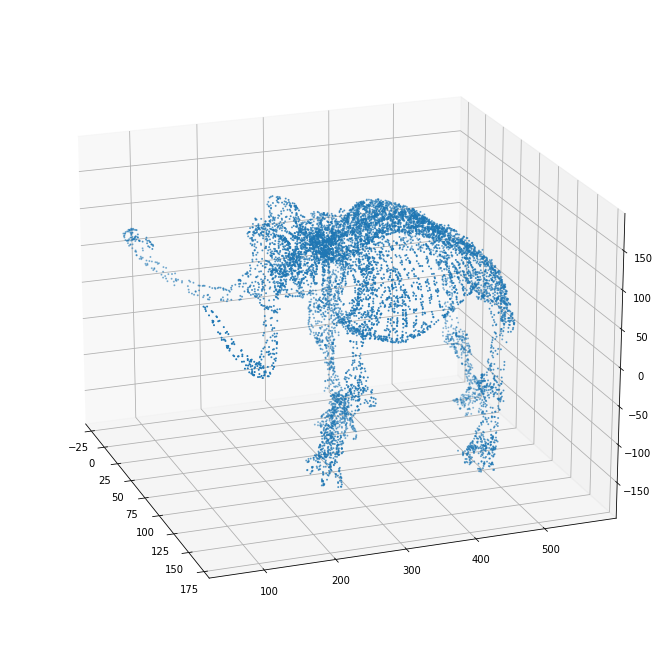
First, let's fetch the dataset that we experiment on. The data represents 3D coordinates of a mammoth. Below we include a figure of original dataset.
source = "https://raw.githubusercontent.com/MNoichl/UMAP-examples-mammoth-/master/mammoth_a.csv"

data = Req.get!(source).body

df = DF.load_csv!(data)
#Explorer.DataFrame<
Polars[999778 x 3]
x f64 [58.823, 59.197, 58.734, 59.043, 59.223, ...]
y f64 [228.407, 228.642, 228.931, 228.693, 228.667, ...]
z f64 [79.843, 77.478, 78.515, 78.571, 78.611, ...]
>Now, convert the dataframe into tensor, so we can manipulate the data using Scholar.
tensor_data = Nx.stack(df, axis: 1)#Nx.Tensor<
f64[999778][3]
EXLA.Backend<host:0, 0.2236801022.581042190.174268>
[
[58.823, 228.407, 79.843],
[59.197, 228.642, 77.478],
[58.734, 228.931, 78.515],
[59.043, 228.693, 78.571],
[59.223, 228.667, 78.611],
[59.103, 228.711, 78.305],
[58.854, 228.786, 78.597],
[59.123, 228.695, 77.371],
[59.002, 228.592, 78.925],
[58.368, 227.879, 81.155],
[59.168, 229.8, 74.95],
[58.798, 229.431, 76.296],
[59.257, 229.227, 76.144],
[58.408, 250.928, 93.15],
[58.575, 250.743, 93.323],
[71.011, 217.179, 62.859],
[70.259, 217.511, ...],
...
]
>Since there is almost 1 million data points and they are sorted, we shuffle dataset and then use only the part of the dataset.
Trimap
We start with Trimap. It's a manifold learning algorithm that is based of nearest neighbors. It preserves the global structure of dataset, which can be used for understanding the overall data distribution. Let's look what will be the result of the Trimap on mammoth dataset.
{tensor_data, key} = Nx.Random.shuffle(Nx.Random.key(42), tensor_data)

trimap_res =
  Scholar.Manifold.Trimap.transform(tensor_data[[0..10000, ..]],
    key: Nx.Random.key(55),
    num_components: 2,
    num_inliers: 12,
    num_outliers: 4,
    weight_temp: 0.5,
    learning_rate: 0.1,
    metric: :squared_euclidean
)#Nx.Tensor<
f64[10001][2]
EXLA.Backend<host:0, 0.2236801022.581042192.174259>
[
[87.5960481212865, 107.83563946728007],
[95.93224095586187, 91.03811962459187],
[76.23538360750037, 101.22665484812988],
[91.28047447374527, 83.89099279844432],
[84.84272736715022, 63.05776975461835],
[77.47594824886791, 70.58007253201106],
[48.1726647167702, 83.59889134210331],
[87.09967163881679, 81.16403134057438],
[78.77111626020424, 89.5381523774902],
[97.90247495971414, 90.30331715233045],
[74.82692937810215, 88.72983366943957],
[84.41794589221618, 100.28068173065604],
[48.9525994243841, 65.31540933930391],
[97.74716685388529, 87.01213386339163],
[55.25583739452793, 78.09500152893669],
[78.8556707294727, 96.20470118706773],
[87.06284966061098, 92.95614239803128],
[98.14345384260274, 77.08288277313781],
[45.61527701121027, 86.90240376974904],
[109.77362315414614, 105.15212699721849],
[77.18580406991187, 90.15798204995377],
[72.62493132684811, 61.503358925355755],
[64.86122257994592, 56.26636625077798],
[107.15238372453034, 86.8502564790939],
[76.74146917610297, 92.78343841441362],
...
]
>Now, lets plot the results of Trimap algorithm
coords = [
  x: trimap_res[[.., 0]] |> Nx.to_flat_list(),
  y: trimap_res[[.., 1]] |> Nx.to_flat_list()
]

Tucan.scatter(coords, "x", "y", point_size: 1)
|> Tucan.set_size(300, 300)
|> Tucan.set_title(
  "Mammoth dataset with reduced dimensionality using Trimap",
  offset: 25
)
{"$schema":"https://vega.github.io/schema/vega-lite/v5.json","height":300,"layer":[{"data":{"values":[{"x":87.5960481212865,"y":107.83563946728007},{"x":95.93224095586187,"y":91.03811962459187},{"x":76.23538360750037,"y":101.22665484812988},{"x":91.28047447374527,"y":83.89099279844432},{"x":84.84272736715022,"y":63.05776975461835},{"x":77.47594824886791,"y":70.58007253201106},{"x":48.1726647167702,"y":83.59889134210331},{"x":87.09967163881679,"y":81.16403134057438},{"x":78.77111626020424,"y":89.5381523774902},{"x":97.90247495971414,"y":90.30331715233045},{"x":74.82692937810215,"y":88.72983366943957},{"x":84.41794589221618,"y":100.28068173065604},{"x":48.9525994243841,"y":65.31540933930391},{"x":97.74716685388529,"y":87.01213386339163},{"x":55.25583739452793,"y":78.09500152893669},{"x":78.8556707294727,"y":96.20470118706773},{"x":87.06284966061098,"y":92.95614239803128},{"x":98.14345384260274,"y":77.08288277313781},{"x":45.61527701121027,"y":86.90240376974904},{"x":109.77362315414614,"y":105.15212699721849},{"x":77.18580406991187,"y":90.15798204995377},{"x":72.62493132684811,"y":61.503358925355755},{"x":64.86122257994592,"y":56.26636625077798},{"x":107.15238372453034,"y":86.8502564790939},{"x":76.74146917610297,"y":92.78343841441362},{"x":88.73778966398886,"y":67.97257318625593},{"x":70.99803196972384,"y":103.39188613708355},{"x":93.8689893409936,"y":80.40775764931409},{"x":63.622325530079415,"y":73.59244242525864},{"x":75.09031640499185,"y":86.83667555455354},{"x":94.32118161115095,"y":96.99325319951942},{"x":90.97666938354884,"y":79.27689751097493},{"x":98.36519242532857,"y":82.14883223121453},{"x":89.12182574623574,"y":105.39656161238271},{"x":75.50710985300917,"y":83.70930124282594},{"x":58.416221421372796,"y":64.8282610660516},{"x":85.47849000871007,"y":62.037443173587945},{"x":105.04342954310654,"y":90.85626816973534},{"x":92.44024682796613,"y":82.9446355081128},{"x":72.18770579584675,"y":58.33625226517835},{"x":85.41067604286695,"y":83.63218606104869},{"x":85.13977486575568,"y":82.84069699550076},{"x":93.67844360402454,"y":79.86742793974868},{"x":76.1343064941052,"y":87.59893252131427},{"x":85.3385769147656,"y":109.57438766198621},{"x":74.60499322523177,"y":67.35188048096728},{"x":73.87830631626957,"y":84.2431097773822},{"x":90.07522143421437,"y":80.04402901897554},{"x":107.13273027217987,"y":79.92735974550794},{"x":41.63445052462818,"y":70.3732373866874},{"x":89.74810027912035,"y":85.92108130198844},{"x":59.46872012638843,"y":65.6811622492299},{"x":87.55291067867516,"y":69.80508085756527},{"x":50.00854806011233,"y":99.86924459115524},{"x":77.33578132814128,"y":81.92606131706786},{"x":68.30139466546277,"y":58.717826039619915},{"x":93.03523091019707,"y":82.72580628985568},{"x":51.89309907687393,"y":93.1526046236352},{"x":92.08877163140052,"y":86.00091539840834},{"x":114.00651182723844,"y":99.52069128843137},{"x":61.568473965591764,"y":65.44660966535082},{"x":44.418105676664126,"y":106.5128962410755},{"x":73.47645907619113,"y":61.72227721244882},{"x":72.37608837638989,"y":79.77261739472277},{"x":85.81115068877179,"y":86.43393253311447},{"x":85.096374153739,"y":70.76234845671118},{"x":91.35094619480286,"y":77.85995767452926},{"x":74.78225441147524,"y":103.25036959991677},{"x":87.22514416517853,"y":72.04094726949484},{"x":85.82238201784858,"y":81.51494014722894},{"x":89.80725255202391,"y":66.95582709069168},{"x":112.96744338350328,"y":98.83491123999511},{"x":88.01556957565259,"y":70.6004633604809},{"x":84.6950695711977,"y":93.43496846198},{"x":87.39298432991708,"y":85.33826487385345},{"x":91.99617443720828,"y":85.97689655825478},{"x":77.60850832538476,"y":76.3729315526922},{"x":89.56366602385025,"y":76.6995378273398},{"x":102.37545327984841,"y":82.21058913980683},{"x":99.4101324653975,"y":100.03903612233427},{"x":73.38109123100065,"y":82.99502346257758},{"x":87.97138725841711,"y":62.17695502600828},{"x":46.78236948615004,"y":102.03002632250072},{"x":63.802123764866295,"y":110.09812744433866},{"x":96.17179761433928,"y":94.474705731106},{"x":65.28772406872933,"y":106.9845717999335},{"x":57.7574744897225,"y":86.08633049449601},{"x":86.40870735191356,"y":78.13127536312227},{"x":89.33291764637698,"y":85.84827221330606},{"x":61.83947464459311,"y":62.54765838246026},{"x":83.20191044668628,"y":63.29156607244424},{"x":85.47054386577047,"y":58.892471654117884},{"x":94.9835103763703,"y":95.92701904738126},{"x":91.50917523697895,"y":85.1020219478316},{"x":85.63707661481737,"y":91.73741763561802},{"x":55.126372253025615,"y":91.93848711038781},{"x":53.723775628976675,"y":90.18265460902316},{"x":78.20534003781982,"y":84.85605944996068},{"x":88.19882438530873,"y":103.6149463733208},{"x":80.77067517665571,"y":98.43194470597338},{"x":87.97296694013421,"y":84.75013988234927},{"x":76.60209004924991,"y":56.23094520104623},{"x":85.907191975236,"y":82.1795983924433},{"x":101.20410478147211,"y":89.27573876250969},{"x":78.27467718968384,"y":86.26954287894091},{"x":116.61874131916073,"y":96.05341157456257},{"x":75.1637539488186,"y":75.90017305793882},{"x":79.20032106959798,"y":86.35706379498532},{"x":97.58514532360348,"y":77.19077418697887},{"x":102.75119198150247,"y":83.06939364539087},{"x":102.67792002399736,"y":88.79738339809212},{"x":86.48038989762102,"y":88.75947523594171},{"x":64.50649913141491,"y":78.70597004251773},{"x":67.5901618602183,"y":66.4634962637037},{"x":45.878716906022824,"y":100.6832221432948},{"x":91.36866243827436,"y":85.45057863484605},{"x":88.7149894247466,"y":109.83120732684989},{"x":100.1994467017181,"y":83.02024603405913},{"x":89.04285361720324,"y":61.961656749210974},{"x":66.74661799237974,"y":109.69250435301537},{"x":52.049047022429654,"y":62.48807501919234},{"x":56.38524175536789,"y":91.74811724857331},{"x":78.13936827585371,"y":79.19936124769198},{"x":74.7002338474629,"y":88.13620077786685},{"x":94.03332649923861,"y":83.22948329545324},{"x":56.51892777957654,"y":91.09081606380602},{"x":106.7678971941715,"y":83.90671700263107},{"x":100.78048625465024,"y":94.24321777701327},{"x":106.52360741655332,"y":87.01357369613747},{"x":81.75573229194636,"y":65.79872725915048},{"x":95.82064380027157,"y":81.78551384934073},{"x":79.32875909718089,"y":79.68537732780946},{"x":82.82096335998392,"y":112.06837544044816},{"x":85.80832226456188,"y":70.2796055879489},{"x":87.55988174433725,"y":91.78495717172886},{"x":91.42168601749553,"y":83.08698541862302},{"x":73.9053839440435,"y":78.02227395035995},{"x":95.15726839996326,"y":67.63287881640886},{"x":100.32982849351951,"y":92.81297125209788},{"x":85.19753642997159,"y":68.51676101909086},{"x":83.48775985807309,"y":83.3330624883833},{"x":91.19924338081061,"y":85.78581470287237},{"x":84.11079701013041,"y":100.96208770906007},{"x":73.84010500360714,"y":78.54744492541204},{"x":104.76924786554899,"y":91.38279902114036},{"x":77.86742443270946,"y":54.84380096564752},{"x":86.71515637281179,"y":75.21997815705747},{"x":37.03898568846219,"y":94.02306125818838},{"x":104.70719612781343,"y":76.7560302559338},{"x":66.50399078972114,"y":65.17622906128568},{"x":72.31394316807807,"y":102.28508451386097},{"x":91.87792951085738,"y":83.06941463417643},{"x":79.77623880668561,"y":66.30813322353987},{"x":77.06125276091461,"y":79.70664139972943},{"x":82.43280315420093,"y":112.09211804799936},{"x":77.51722166130783,"y":64.41532416054027},{"x":98.45270086317547,"y":91.44538546839219},{"x":104.30989085184142,"y":100.64046596679285},{"x":74.26534977994413,"y":71.28351307784631},{"x":72.36186882456637,"y":82.80796706975765},{"x":98.026152432385,"y":82.16434264162922},{"x":72.69512313375168,"y":75.70856409652176},{"x":82.66044608897407,"y":111.45296449179044},{"x":79.00579323822778,"y":69.12950616436724},{"x":87.28735969047774,"y":108.75738096111486},{"x":90.2801666017389,"y":89.46513620924067},{"x":46.636464364386214,"y":71.48179487697494},{"x":87.8659277734153,"y":65.4454233618212},{"x":107.2518720037445,"y":81.2835391011905},{"x":72.81949109790263,"y":65.15064780217696},{"x":44.68391391391651,"y":105.61251268413169},{"x":91.03165248956911,"y":86.81664776569043},{"x":45.56370346740899,"y":87.82840764404197},{"x":89.40228349764351,"y":80.51402303078092},{"x":88.08163204799875,"y":65.77686567295613},{"x":37.716989313630954,"y":76.75506085268711},{"x":87.98721247653263,"y":104.84447728586476},{"x":88.42070511289543,"y":109.85643530660502},{"x":104.56262899259343,"y":105.72865401079558},{"x":69.38530996915412,"y":106.73197064743405},{"x":62.18562002088994,"y":109.44725881527852},{"x":77.5312030542321,"y":55.51447541491913},{"x":56.82103813249563,"y":91.07172344300831},{"x":44.92793761226791,"y":87.27092750568183},{"x":94.28003070801205,"y":78.46220129903271},{"x":94.05665326994159,"y":76.71707737120036},{"x":78.93395874478475,"y":69.10655895337337},{"x":79.28554442097533,"y":92.3519804019819},{"x":90.61223830160326,"y":68.61285233554923},{"x":78.02950210947326,"y":73.93623817059216},{"x":81.18745117257713,"y":95.86284845148249},{"x":88.09286003063215,"y":70.38738166553458},{"x":99.58231484158115,"y":78.26712409453948},{"x":105.35118931716211,"y":90.86030515914254},{"x":51.65163751369193,"y":93.03422971568577},{"x":73.6754855212219,"y":104.44554954255244},{"x":89.66745454177854,"y":87.51840445953137},{"x":104.34893390232823,"y":106.47203567327152},{"x":79.25424758172613,"y":79.7345692895212},{"x":79.87345718881387,"y":59.049738632527614},{"x":83.0668086600405,"y":72.5507735180603},{"x":73.3437845686259,"y":101.45432701971633},{"x":77.80795277079373,"y":75.00726157896537},{"x":77.49529472089748,"y":54.817235197122784},{"x":100.5926730270648,"y":95.74285477348201},{"x":70.1744154184505,"y":104.99133171133083},{"x":46.98505783578923,"y":86.69100772325531},{"x":37.3646030541515,"y":95.10778420793834},{"x":47.030709876182925,"y":71.20823102927997},{"x":85.98636841946866,"y":68.92731203642931},{"x":63.28272351115463,"y":110.85547410735319},{"x":56.13455852699788,"y":86.98960402751746},{"x":78.79776481136223,"y":65.84183042426497},{"x":61.952222400260126,"y":74.42326643890081},{"x":80.9436943692025,"y":58.7676148274888},{"x":88.25933673384712,"y":91.98195426370157},{"x":80.33221682233959,"y":88.30848780874318},{"x":42.46530679999071,"y":85.92552256079478},{"x":84.10268828396646,"y":110.03618206103823},{"x":51.13065956361847,"y":102.68574396226776},{"x":87.15492204828612,"y":65.34136023127552},{"x":78.64915092924646,"y":69.86510245030942},{"x":84.07501607479728,"y":75.03959826125714},{"x":85.91066495688818,"y":87.30168714936154},{"x":94.59321309153461,"y":80.24562785812965},{"x":79.17575356514674,"y":91.11044655365882},{"x":84.6022754293652,"y":80.1402771883383},{"x":76.75953324603695,"y":71.59491655496095},{"x":85.54976654920326,"y":59.80574510144842},{"x":39.09648329899879,"y":93.6197001532121},{"x":83.57603993574058,"y":110.76805736097515},{"x":88.80303220351362,"y":82.49574413839956},{"x":67.44797646210469,"y":65.482252561445},{"x":86.92803339844822,"y":73.12465286085475},{"x":43.78432164188236,"y":105.95088325794765},{"x":86.86494367461889,"y":84.89482944011186},{"x":88.38370738325844,"y":105.51243695257591},{"x":85.79235438444421,"y":92.03091199328836},{"x":95.00859159186305,"y":92.62126524838261},{"x":48.83678222917835,"y":101.88833993719378},{"x":85.94964150655167,"y":87.94517371497076},{"x":103.97126402911806,"y":84.46312887313502},{"x":86.10213651616678,"y":78.63827223165048},{"x":114.5319246853433,"y":98.5718402554184},{"x":77.87102254187559,"y":86.77678283340785},{"x":87.80427388740672,"y":102.97031402863571},{"x":78.2490238494676,"y":97.8613686468678},{"x":50.94361195390674,"y":101.4825088366759},{"x":97.49661711953127,"y":99.4073132846398},{"x":74.62296206004086,"y":85.40457342524151},{"x":37.831707128413164,"y":76.20483879250644},{"x":86.1981279027642,"y":90.68235050725191},{"x":74.19682862698549,"y":58.3795277412584},{"x":67.9842875927561,"y":109.31401050697612},{"x":87.66473752359737,"y":109.05966934056303},{"x":92.05620453122046,"y":80.39950842730208},{"x":60.6528534487724,"y":110.25568355297274},{"x":80.30445046850838,"y":69.9788895584206},{"x":78.64249677838035,"y":89.04196137403657},{"x":105.82527599238917,"y":90.48825484659008},{"x":55.147780934292136,"y":87.4247976271712},{"x":94.82438766524956,"y":70.55931711609162},{"x":80.55391321104116,"y":110.75355973317997},{"x":78.16944227504432,"y":61.122481742379215},{"x":111.1032899611564,"y":99.34265847452774},{"x":83.0714124202196,"y":114.08044765901597},{"x":88.48293425865344,"y":76.38462003371629},{"x":101.70417474424053,"y":86.63049686497334},{"x":91.68808079317863,"y":81.63707111151795},{"x":67.96733824210325,"y":57.95745688799609},{"x":75.68572709528905,"y":102.3275065129881},{"x":91.00261962585654,"y":80.80518942953854},{"x":80.33236241985864,"y":97.16034238341283},{"x":57.89956076589774,"y":85.89908448882494},{"x":78.22066588131116,"y":91.75891279159748},{"x":86.52989515033062,"y":82.90139215658745},{"x":100.15793739905678,"y":95.50885816986138},{"x":97.75879085625061,"y":78.27823053864456},{"x":99.8833021725575,"y":96.5472124717659},{"x":93.93197314956134,"y":78.45031537840337},{"x":76.85581772687483,"y":77.10110290338768},{"x":86.26251435386001,"y":88.05649529343974},{"x":95.33328512886307,"y":81.37645930452506},{"x":77.75966727520904,"y":58.69954305735076},{"x":84.68293419874678,"y":90.07164381455732},{"x":67.33963943169195,"y":56.69344914764936},{"x":88.08683892487856,"y":110.51814907399863},{"x":107.55205084534434,"y":85.0983396052875},{"x":94.70304602471886,"y":77.05220398455404},{"x":84.859341601617,"y":78.90413026701033},{"x":89.46371640918971,"y":92.1057652964282},{"x":98.63538393799334,"y":100.13602154357335},{"x":101.39964258105688,"y":83.31612794098596},{"x":89.78941676298932,"y":78.75005069979754},{"x":75.28016749611602,"y":66.49996121516779},{"x":82.1449689316453,"y":63.10719774337256},{"x":94.95984508196801,"y":68.43832431874299},{"x":75.55080992221528,"y":100.56751742499115},{"x":72.92972797034902,"y":103.89039031101984},{"x":74.81472213652927,"y":73.07295625304423},{"x":97.75480250888222,"y":97.94464219037236},{"x":86.05466991709551,"y":89.59426160328044},{"x":115.54415241893555,"y":96.60496655869912},{"x":86.13378484355086,"y":91.42162126256646},{"x":79.19359049185896,"y":54.326987101115705},{"x":82.44723186841067,"y":63.74882513667451},{"x":95.48227480474509,"y":77.4692181067564},{"x":87.64813772942821,"y":80.98704233165813},{"x":90.01444863331528,"y":73.50630050834349},{"x":45.10844028219565,"y":101.25223374945249},{"x":87.92096171246855,"y":65.42703750665031},{"x":110.83386929125086,"y":99.34094336031352},{"x":59.676208739675815,"y":63.98467717277842},{"x":82.2699653881818,"y":71.8807008950826},{"x":67.1896084351727,"y":108.43141849697713},{"x":109.83410173248951,"y":99.54434653286825},{"x":51.18067762706112,"y":98.64706064231115},{"x":98.432166437516,"y":94.64233337718018},{"x":35.50599032487314,"y":95.82925074448309},{"x":53.70870348747744,"y":81.36421321883125},{"x":94.71117432374571,"y":92.63120959169225},{"x":64.27854548744358,"y":60.36032018657464},{"x":83.92473953638428,"y":67.68804691642532},{"x":94.51251987656572,"y":89.53955365415612},{"x":106.67719221989876,"y":86.61652938665043},{"x":89.16318048344465,"y":87.3001428512784},{"x":68.50913485164257,"y":56.54084709477633},{"x":92.3994564705441,"y":79.18554219224941},{"x":49.51894125987529,"y":104.82348191607454},{"x":63.99845007483854,"y":66.49710026442591},{"x":102.71213847333364,"y":83.2409204673008},{"x":55.43016224410593,"y":89.83110012748082},{"x":90.55466813036203,"y":76.57299952788851},{"x":85.93338807734433,"y":98.46484500566972},{"x":86.62591080476385,"y":86.43237592762601},{"x":80.39928652185586,"y":57.021943030172594},{"x":94.28688813103504,"y":81.81801792387269},{"x":92.99094215934235,"y":73.73286118866233},{"x":103.15870796064655,"y":80.07509512169102},{"x":105.84336669174431,"y":78.21844543595755},{"x":102.18983110738797,"y":90.28608839008884},{"x":94.1509188690751,"y":93.18419284941149},{"x":73.49824403110048,"y":73.86201044755633},{"x":99.498066937601,"y":82.45721885674642},{"x":88.25116551034381,"y":89.26255576964384},{"x":94.93538170371573,"y":88.16451749197361},{"x":101.74589206436438,"y":88.43833669680643},{"x":80.835656675433,"y":98.34011135486091},{"x":94.84369670967479,"y":67.91630408911782},{"x":75.5524599630459,"y":84.49060148974463},{"x":86.95276881136702,"y":85.20136216935168},{"x":78.63614021986368,"y":68.55247668006197},{"x":101.00578777573931,"y":88.34217004719599},{"x":47.285619552233015,"y":102.21205095922537},{"x":72.12889188630363,"y":62.823924247871076},{"x":98.8442436213085,"y":81.049777667139},{"x":33.51464339446447,"y":97.55078565865519},{"x":37.90454175895504,"y":89.97557668351395},{"x":87.62900848536721,"y":91.0880001791697},{"x":101.3466735169288,"y":84.82275174384208},{"x":84.85283928203344,"y":99.45738790020347},{"x":76.22388246115369,"y":63.349902320286304},{"x":105.12631723365168,"y":80.62083715160878},{"x":77.14149644641972,"y":81.51877664203909},{"x":81.47176164962005,"y":84.60450625679846},{"x":47.54892194674852,"y":83.70117638445114},{"x":93.07103021878243,"y":80.42843166101483},{"x":86.56364658879252,"y":79.53869781286491},{"x":87.60956114251098,"y":94.90382908264763},{"x":86.51536661613484,"y":88.4130917167929},{"x":77.34346006895179,"y":93.18969306241628},{"x":81.81917399747377,"y":85.6295137451786},{"x":76.42861747578355,"y":56.43019755124079},{"x":99.65519935847107,"y":99.77028633389945},{"x":72.3069524739094,"y":105.22648927689497},{"x":96.50848828103317,"y":98.81423954171342},{"x":85.30154963057305,"y":93.05563173237917},{"x":79.93984032618359,"y":87.26941960919784},{"x":76.31483391945689,"y":76.03238051251196},{"x":68.49576969113274,"y":58.163333295555546},{"x":58.804480248114714,"y":79.11928719750209},{"x":87.81721781236703,"y":81.11305727621847},{"x":75.52764403541119,"y":87.22356058925966},{"x":77.41243992480703,"y":68.64403927294022},{"x":46.84845635345924,"y":71.09161698135814},{"x":46.815275296910116,"y":101.92792343568598},{"x":44.20341251920962,"y":83.05397464015424},{"x":57.11472993606107,"y":75.35110628932172},{"x":84.17483518976061,"y":97.9611453299918},{"x":96.95381333780657,"y":90.76731703111793},{"x":90.31067951573421,"y":88.17184571433795},{"x":82.38743249200729,"y":56.47749233636247},{"x":59.56731056632643,"y":73.29472009928108},{"x":90.57789626233387,"y":64.35957356038425},{"x":90.16722650512291,"y":79.27998884977342},{"x":81.39782016518089,"y":81.92294625643457},{"x":88.45044586257983,"y":85.69287468470509},{"x":63.64455059330389,"y":67.09361545663765},{"x":46.02256258803292,"y":84.917638893558},{"x":77.56589759402509,"y":61.69280252736737},{"x":75.35105518114568,"y":64.12325581037557},{"x":49.576252170847816,"y":76.577132422991},{"x":64.44441816205494,"y":73.1110864790388},{"x":84.85540040013493,"y":91.02917075045379},{"x":97.62342789954968,"y":89.33716442535444},{"x":99.3602135163362,"y":91.54268396967845},{"x":86.27759744598232,"y":60.29098721602885},{"x":82.0406658230153,"y":89.66874638474059},{"x":85.96523986617058,"y":84.1724288746616},{"x":78.67078668382263,"y":54.589791431516446},{"x":108.61663703382837,"y":105.65489279242995},{"x":94.08554803432108,"y":97.05853442607695},{"x":96.86528172363118,"y":88.02388249516198},{"x":74.96002692338806,"y":90.27726756961651},{"x":43.677360016153216,"y":89.52420227842568},{"x":77.2048252169399,"y":101.14287112903797},{"x":82.75828359050792,"y":57.161136585736294},{"x":56.653686723033665,"y":73.1667461409288},{"x":68.22766891633512,"y":108.12386102341029},{"x":92.76395093237002,"y":81.71389970939462},{"x":68.35972069605641,"y":62.604881118740316},{"x":90.21942802977257,"y":83.25746529314033},{"x":67.25829710704544,"y":58.18760580603765},{"x":82.71112651297808,"y":75.53696515452009},{"x":63.64566305164259,"y":62.71405153237462},{"x":111.84930460947254,"y":105.80004108194069},{"x":94.52393084729482,"y":74.4837924617662},{"x":72.69842875655354,"y":78.8064378661997},{"x":99.60206631108683,"y":96.62085981446845},{"x":84.52405757771157,"y":60.14270208938762},{"x":82.78978400554374,"y":95.12240751076216},{"x":85.60630318560726,"y":98.98030356258289},{"x":87.08008872133068,"y":71.27524939149757},{"x":87.91088960721956,"y":94.7470254439625},{"x":79.39837829462085,"y":68.65850957902762},{"x":81.17520125393791,"y":109.95771035768566},{"x":106.71437638158653,"y":83.8878280900412},{"x":52.96594845296531,"y":65.4067843174755},{"x":66.52529912421376,"y":118.18342777826413},{"x":87.49429943614089,"y":102.61566459062692},{"x":94.91036531904709,"y":81.5250358009913},{"x":104.30599065730863,"y":75.83226867213176},{"x":86.96764150123381,"y":80.53683483521358},{"x":39.29711486240446,"y":93.39120496598157},{"x":89.62526799955592,"y":81.19780524759985},{"x":105.93786838693451,"y":77.84245261298969},{"x":90.32970171515798,"y":88.41377904048679},{"x":97.63252380525242,"y":77.78825082879415},{"x":95.52936452287723,"y":79.84036709087474},{"x":87.9076203295659,"y":63.45466944522734},{"x":43.542419948786566,"y":106.42151572269437},{"x":79.47319285625841,"y":111.0949118566261},{"x":86.35249188195955,"y":101.81410729827144},{"x":106.8840247458705,"y":86.36704596701587},{"x":97.89672790238384,"y":79.1080482749706},{"x":104.27141051296637,"y":85.267661433699},{"x":80.35679795000205,"y":77.66374894311924},{"x":76.26970731575084,"y":82.55435331878522},{"x":43.70164432520604,"y":73.37263260898018},{"x":88.00511687544585,"y":61.7376915840397},{"x":88.55090854338425,"y":61.87875554074766},{"x":46.338803579199215,"y":109.14283227384713},{"x":87.40571051303611,"y":85.35845818670411},{"x":85.66097204239622,"y":111.20223905248115},{"x":103.81459929124726,"y":88.1378954226592},{"x":83.5883127172796,"y":82.21142860499495},{"x":54.070070994825926,"y":63.62052275567102},{"x":85.54068956898263,"y":86.68040232793146},{"x":70.63608819317608,"y":103.75565980819596},{"x":77.2253368508151,"y":70.52993731132116},{"x":80.18427598007203,"y":109.77546642289704},{"x":81.21963275869419,"y":112.27940022527466},{"x":51.253243758764604,"y":82.22923381257363},{"x":72.8054366585096,"y":61.33756149645193},{"x":91.32444714905978,"y":81.70186892277495},{"x":62.3594499354372,"y":73.14395189900102},{"x":89.31319787808503,"y":79.07916289539241},{"x":72.61164398534231,"y":74.10113920305801},{"x":81.001579350096,"y":59.59209780381918},{"x":71.57897683486874,"y":63.46464924389617},{"x":76.45515940336615,"y":77.24213787859232},{"x":93.4913110503681,"y":76.8607770944153},{"x":92.37134793004046,"y":62.740496832872054},{"x":106.0311523655369,"y":76.61002293037873},{"x":83.2311212021596,"y":59.077716133168714},{"x":89.18055685317724,"y":106.84563402954507},{"x":61.02130189260344,"y":76.72604238573935},{"x":79.5714735491005,"y":110.47481468679123},{"x":76.18001930912618,"y":65.71392186694045},{"x":66.04643749371269,"y":58.960278636951514},{"x":38.19523777043335,"y":90.12881352516962},{"x":40.74348168857047,"y":91.43018944622854},{"x":86.66781432800039,"y":63.82617251849709},{"x":88.50274746422777,"y":73.1224017930531},{"x":64.48547563826897,"y":105.69300984617249},{"x":60.23548134941183,"y":62.02212382574673},{"x":109.76384150963254,"y":105.5569850197413},{"x":84.72938830392944,"y":93.48194324442915},{"x":80.8490792755472,"y":71.04295692603036},{"x":90.31642176598773,"y":78.75902953944569},{"x":49.697325084015034,"y":105.68363218628197},{"x":41.63680102247774,"y":70.69009872660625},{"x":77.94879392699677,"y":66.82451870547396},{"x":61.49077928294074,"y":108.82557204840913},{"x":105.41112096491987,"y":81.24855477107786},{"x":77.0699150552354,"y":60.38086159712284},{"x":103.56168537284644,"y":75.36685389914982},{"x":89.82136272221348,"y":68.30506864985382},{"x":65.65476794261494,"y":58.10058250596935},{"x":63.845079578360114,"y":58.62114413334064},{"x":105.65113044258887,"y":75.76177313033484},{"x":88.68052824020756,"y":69.2588054594185},{"x":103.64944371440536,"y":101.07732504470269},{"x":100.42077049463346,"y":80.45217554247745},{"x":86.33289056429746,"y":59.4394603661458},{"x":60.07010553633618,"y":66.7067046877864},{"x":49.38410443105873,"y":76.73274007425111},{"x":75.02954980481344,"y":66.78115296025172},{"x":96.6241261995132,"y":87.5331382623282},{"x":63.053689930765074,"y":70.99632905900837},{"x":74.60594480177348,"y":79.95466510405129},{"x":97.7513792361786,"y":85.89132523585826},{"x":88.13365122968447,"y":90.11838061549145},{"x":60.74488267116015,"y":105.71041770902379},{"x":77.2413163797536,"y":54.55556664658457},{"x":53.06759352671288,"y":95.33551198725034},{"x":75.80906743766448,"y":100.54382198797984},{"x":98.27963613580526,"y":93.2983658446517},{"x":96.55396061963495,"y":101.69094991495463},{"x":76.59036916583149,"y":75.19127597812712},{"x":86.46969922010908,"y":97.2548302388897},{"x":94.02604186026551,"y":69.63482005396988},{"x":108.44852752099682,"y":99.49797488980832},{"x":64.98531893691272,"y":56.240188423987505},{"x":76.89639617805388,"y":72.59611363387005},{"x":45.438627326954716,"y":108.77079303813227},{"x":67.6801424340544,"y":107.55513144898583},{"x":96.76671269086405,"y":82.50925774696738},{"x":90.83631628132565,"y":69.44071884123252},{"x":77.59952734448176,"y":86.96682462366196},{"x":49.33747472574773,"y":106.45474312346262},{"x":77.17895474539081,"y":93.23096589201673},{"x":55.55157491819628,"y":89.28516111410364},{"x":94.988415922994,"y":74.70586569083409},{"x":91.92086104685842,"y":80.54358118266005},{"x":79.66115152266711,"y":96.91511707720251},{"x":105.14679992154416,"y":80.20326893896075},{"x":100.99076493185835,"y":81.52714721560149},{"x":87.16428437333049,"y":78.7273448797657},{"x":84.86261944775647,"y":109.67398189329272},{"x":97.99663822855206,"y":94.4564817724796},{"x":86.23634506275656,"y":86.71310534715572},{"x":90.12078497305853,"y":76.94447648187081},{"x":88.618504970719,"y":84.71592988827953},{"x":80.07590273006244,"y":97.73889984679982},{"x":61.23920559222496,"y":76.106626484846},{"x":77.38168827518426,"y":55.14507753220939},{"x":78.72303410870038,"y":59.4536467390861},{"x":101.79683767896366,"y":88.9617636955257},{"x":56.420672044856154,"y":78.9326099962333},{"x":77.18832936268886,"y":64.31658107471718},{"x":75.52213400731384,"y":83.44742681245408},{"x":74.89487279183999,"y":55.04795140914018},{"x":98.54724250181621,"y":83.35602284754897},{"x":99.047679151603,"y":86.71558991846773},{"x":98.41408847557568,"y":81.85046446095211},{"x":87.64444317864374,"y":75.04464637920303},{"x":83.36046647030092,"y":92.8779784007467},{"x":86.9595630500511,"y":87.88305841666929},{"x":101.78456684131471,"y":91.94903040691685},{"x":105.27182327453508,"y":84.96771723087713},{"x":85.86146616592501,"y":111.44526207030104},{"x":94.74671374390482,"y":92.4974223821977},{"x":83.68826285757406,"y":59.49107813812191},{"x":88.97689384522693,"y":73.0248096357013},{"x":59.422929941923705,"y":77.9497241640688},{"x":39.303057828078565,"y":90.23165764896939},{"x":74.32336948870919,"y":85.1721142744212},{"x":76.39587957183299,"y":100.89854558413472},{"x":73.05853359589435,"y":71.25404701492616},{"x":82.65782578396544,"y":69.3837423652004},{"x":107.06521507762994,"y":78.318105175718},{"x":58.52770059171882,"y":79.23101506053717},{"x":87.4536057033124,"y":78.43192845235758},{"x":71.37441058181143,"y":103.4916687971154},{"x":89.30812434656855,"y":66.31642405350193},{"x":87.65964223163529,"y":83.29517523867626},{"x":88.5735024432169,"y":87.23281476337125},{"x":80.36037268127355,"y":58.99900640655298},{"x":85.81739025307631,"y":75.7172134582419},{"x":105.22741296101033,"y":75.67337611097362},{"x":60.962812931069514,"y":65.31191275707494},{"x":55.74963159648428,"y":79.28644088023975},{"x":51.856117907800446,"y":80.16092124565641},{"x":80.1877472297894,"y":110.08194911129588},{"x":83.66671005349839,"y":83.98156935497303},{"x":87.89207030234887,"y":89.8045167657598},{"x":47.412673777501126,"y":104.79153979607334},{"x":98.20938509171305,"y":78.31792285852158},{"x":91.90607571986013,"y":83.38217527946594},{"x":84.97502799692964,"y":109.15374795819876},{"x":69.76403070683811,"y":103.9604000696486},{"x":74.1149721304354,"y":83.90889578063552},{"x":63.08542729522877,"y":62.95464163158132},{"x":80.25838261401361,"y":98.7536548647684},{"x":72.25986813211105,"y":73.81199896526041},{"x":56.11807484735374,"y":74.52850996581904},{"x":93.17281424507559,"y":83.50910806638528},{"x":76.80797648023109,"y":65.51785298170746},{"x":106.43823165916785,"y":88.00592527959576},{"x":104.20538465432182,"y":100.76595969683953},{"x":86.40927509896161,"y":72.89073662227284},{"x":42.70980381378325,"y":85.33258384913493},{"x":99.00664396033817,"y":94.05452745809782},{"x":79.81064422640605,"y":57.331027473211876},{"x":56.7952786738592,"y":64.07831897657454},{"x":78.8378911693856,"y":84.41502450911045},{"x":83.5674700874957,"y":109.75236039160622},{"x":43.438046676676294,"y":90.04365121764818},{"x":91.57342125782404,"y":80.67565519162213},{"x":63.79772738304947,"y":76.1484549560413},{"x":85.02085645636699,"y":62.368560404101046},{"x":76.53790151005694,"y":83.11842275499176},{"x":64.97409846195009,"y":78.23049237128076},{"x":101.44159932082523,"y":82.33635433931921},{"x":97.4682444492293,"y":88.57176876857753},{"x":73.80763596704456,"y":76.9381040454053},{"x":79.54016993549106,"y":96.70381441110483},{"x":53.21916747384946,"y":64.93422434381944},{"x":45.516548837211644,"y":87.75959918989767},{"x":83.59052389841045,"y":62.68598202212729},{"x":85.93449488356423,"y":100.7451466052813},{"x":61.12537939292299,"y":76.65575486946517},{"x":84.02184565133115,"y":92.41517092561563},{"x":93.97759806702511,"y":93.49464257965417},{"x":92.54637120439793,"y":84.09532475297061},{"x":88.13616857301264,"y":105.07401996192652},{"x":61.677385507709744,"y":107.3836313995722},{"x":115.76562301534274,"y":96.45071497524849},{"x":78.39316984267397,"y":57.186426677635566},{"x":38.637147113914956,"y":92.83424509735283},{"x":98.19296525236548,"y":85.19906334180534},{"x":79.16870719781207,"y":65.35353258483627},{"x":104.03928590195898,"y":106.23601988143312},{"x":82.68326950981334,"y":74.42899233662266},{"x":66.28386418589993,"y":106.52121986143102},{"x":65.35565000668876,"y":106.03349450532446},{"x":77.60628878515247,"y":57.102391813000466},{"x":50.763137812973426,"y":75.38449538685222},{"x":56.34294682276238,"y":62.57047063708895},{"x":98.24035855629319,"y":91.41952295703001},{"x":63.13522551287397,"y":63.79895069049793},{"x":74.85422385629298,"y":103.09670222896337},{"x":61.063716241741204,"y":65.50193447197306},{"x":49.92571953490937,"y":98.78948905468356},{"x":76.35473028906112,"y":89.76200084232424},{"x":78.43267881279185,"y":54.30902063579319},{"x":99.88286015344767,"y":78.69877073074726},{"x":67.80181378494404,"y":63.03966847148643},{"x":83.14346647099197,"y":82.38980942186643},{"x":50.73852350590311,"y":75.22174510163501},{"x":103.41281300230733,"y":83.68263069457598},{"x":103.5593976152741,"y":106.16058233204988},{"x":74.83333110545074,"y":70.46418471505143},{"x":66.44478383957428,"y":117.58812957203074},{"x":74.96343130617561,"y":85.91826291341981},{"x":78.1829431851657,"y":92.47110963807843},{"x":101.10791339609877,"y":89.35165814970904},{"x":100.38420804332763,"y":104.55372926879663},{"x":87.97033294588266,"y":94.86882538657491},{"x":85.29046473316815,"y":60.64197250783708},{"x":92.10645384017839,"y":62.03112127199059},{"x":86.38722851604837,"y":60.199896877123436},{"x":85.11939316818103,"y":97.49097666178484},{"x":51.850277395688074,"y":62.33419232593381},{"x":61.337390758219385,"y":75.09826086795759},{"x":85.11650440408474,"y":98.50385884519116},{"x":76.18528371941221,"y":75.77103735098626},{"x":75.01674495237714,"y":72.56742798673714},{"x":88.90740181268336,"y":80.95374361678988},{"x":66.94441584690595,"y":108.75269015013356},{"x":88.24620788524636,"y":80.292936140082},{"x":80.95399870941971,"y":76.02527022949374},{"x":95.29272393548732,"y":80.31225882566083},{"x":98.85600873069652,"y":93.84871073954055},{"x":100.67027642809906,"y":86.41994709505114},{"x":86.80382851616037,"y":57.85112984493083},{"x":81.00685174711148,"y":76.21659460440999},{"x":88.17400133065004,"y":83.45646462959853},{"x":97.35275060836183,"y":89.21010360942527},{"x":66.72230443186119,"y":108.28112731584919},{"x":91.08430047952723,"y":71.61409119384993},{"x":69.016914693469,"y":67.47634683098573},{"x":86.69770173832012,"y":87.79828933428422},{"x":78.67495431717408,"y":64.02792823580631},{"x":48.074202414172404,"y":102.7936167605759},{"x":82.41916913576,"y":65.112974992797},{"x":75.05138694605843,"y":86.48353095433075},{"x":80.93614673179053,"y":113.30820916467262},{"x":82.03094154016446,"y":93.09613728960802},{"x":84.51874235877256,"y":89.06958963648712},{"x":91.1980746141378,"y":79.49664930238094},{"x":72.7047270583189,"y":58.12171684106365},{"x":50.36142131821198,"y":75.09558563135978},{"x":37.87385103625816,"y":92.8773287943459},{"x":49.02776179040936,"y":82.73091929275857},{"x":72.3994150863402,"y":60.51505926609068},{"x":97.84388679749839,"y":89.50574522393663},{"x":45.51025592183809,"y":87.98188951031442},{"x":106.503764630227,"y":87.0443542743967},{"x":86.27511010143402,"y":96.62308367851801},{"x":112.03269189105056,"y":99.23668236127615},{"x":85.39480092822723,"y":89.9204124688141},{"x":69.00616308948732,"y":57.540740441497846},{"x":80.47119371432743,"y":85.6674677146591},{"x":68.30970676806827,"y":67.16936471461666},{"x":93.87799890282486,"y":89.35142687179777},{"x":76.51181134006394,"y":54.94254130042217},{"x":83.00231836347535,"y":114.52881233848024},{"x":73.08746116814952,"y":104.2526288579289},{"x":63.72733357256298,"y":56.50305626329029},{"x":57.42621770758299,"y":81.43914252006391},{"x":68.41644856972289,"y":58.76049093922742},{"x":87.24351484918499,"y":82.91133531889686},{"x":58.05516126596846,"y":64.01727041928875},{"x":105.29460160735213,"y":80.74818262316748},{"x":87.15641000349802,"y":82.74292371137852},{"x":91.27597850043811,"y":81.37008555321334},{"x":48.242778654048486,"y":83.15757653594683},{"x":75.00919673952407,"y":103.1878300178635},{"x":85.68661167328989,"y":79.44739643323437},{"x":62.93755615750699,"y":60.08628869712596},{"x":79.72110691197423,"y":55.9182902064475},{"x":74.2804869694373,"y":65.36562570122163},{"x":88.37575775389142,"y":89.90180664434907},{"x":43.53976194529628,"y":73.82421958863804},{"x":51.44418438469225,"y":102.31706255893327},{"x":106.21070050096324,"y":78.8702897205419},{"x":89.18793300791219,"y":81.58631109849097},{"x":79.52276926969533,"y":58.97632780822153},{"x":95.71077617770716,"y":80.06897185865876},{"x":78.8230235160881,"y":87.40217751523002},{"x":33.35649600320626,"y":95.69438539654847},{"x":38.0046110700564,"y":90.08269326049223},{"x":80.37076087504413,"y":75.04184385417028},{"x":97.48450201326294,"y":89.13019739099178},{"x":99.24176729529597,"y":92.10255179721527},{"x":85.32243017824608,"y":100.98250280482767},{"x":106.8176721083584,"y":81.92974351287839},{"x":81.69216819049936,"y":66.71181508993224},{"x":107.93019446079126,"y":85.29565973057124},{"x":47.09054360271787,"y":83.36513422814014},{"x":90.1346340845686,"y":67.77410183229394},{"x":94.81867835122202,"y":77.28577330621731},{"x":94.53064292734308,"y":96.735261448506},{"x":96.20444289562205,"y":82.43199247687006},{"x":79.140006175256,"y":92.1454805017954},{"x":45.14678367995441,"y":87.08786961916417},{"x":81.53892617683951,"y":65.68655178123983},{"x":76.08033184242805,"y":73.97625901727093},{"x":83.57999026825689,"y":76.11246144728116},{"x":81.40236538710276,"y":56.92398489569385},{"x":106.36645780710366,"y":87.41203294409439},{"x":97.69131648604005,"y":86.95280217235948},{"x":88.43638642595167,"y":107.20219754304625},{"x":78.31560994397553,"y":55.104701915785064},{"x":77.76547514597651,"y":55.26381519241057},{"x":77.5382248401269,"y":85.52902065233923},{"x":95.449079834633,"y":82.99454735600318},{"x":105.13892256607859,"y":86.83574959805361},{"x":92.631774481826,"y":79.60496253509285},{"x":56.06344276472128,"y":78.98492027359352},{"x":105.40393189375214,"y":100.51545273288407},{"x":90.18822863179678,"y":77.85969973752665},{"x":83.13831794810696,"y":86.5277710572436},{"x":94.42582434668314,"y":81.97486939279894},{"x":106.85332828575262,"y":81.98089059563827},{"x":64.93017237654497,"y":60.52513561807003},{"x":55.99074525702821,"y":72.32604965839921},{"x":55.57385019392861,"y":63.32766801910007},{"x":44.989371471648376,"y":87.53516875583172},{"x":100.4794338081207,"y":77.41184809883592},{"x":49.96516551365782,"y":106.21996023735468},{"x":90.53650028409065,"y":68.38196893017589},{"x":96.38391070638282,"y":91.18683162393336},{"x":49.531745271618036,"y":98.30496130352728},{"x":57.22719856333547,"y":81.95524875297586},{"x":51.40064489623368,"y":61.138960872572504},{"x":81.4579415074574,"y":97.981965159266},{"x":74.41455024227325,"y":90.28573112828839},{"x":78.3409931526549,"y":64.63122634176699},{"x":77.08546406169641,"y":54.26062300114886},{"x":75.2816256402785,"y":77.9533712977088},{"x":97.40883571957158,"y":102.90619817852951},{"x":62.99220480657869,"y":73.81938853329835},{"x":45.72390236941202,"y":108.43818999196304},{"x":71.28167183281067,"y":71.65857283460818},{"x":100.60320863471732,"y":93.13523770214405},{"x":75.89322007509175,"y":87.1581914002439},{"x":48.61292878360813,"y":66.52743946010636},{"x":60.20335626381882,"y":71.00328832423212},{"x":79.09479929724392,"y":79.73996103675357},{"x":95.00722664720237,"y":83.68097068269782},{"x":104.5461441717068,"y":88.89417290761973},{"x":82.06183960348902,"y":78.81982668975802},{"x":41.26188960433946,"y":92.41073380658905},{"x":104.04541749730359,"y":90.72109430328975},{"x":85.66635304736313,"y":87.98411927304912},{"x":90.7255470618258,"y":88.88397073591942},{"x":62.40891937635393,"y":70.86671447361869},{"x":89.97714114930302,"y":72.99285113756115},{"x":90.83533288263385,"y":84.44359410869565},{"x":59.92605203627833,"y":105.58632239138369},{"x":55.84007509780414,"y":92.32839784358394},{"x":73.96272546225734,"y":65.04622894405308},{"x":92.36205698433542,"y":80.47446461558766},{"x":95.43147016239564,"y":84.01439441785632},{"x":106.77849827984885,"y":82.26786197130897},{"x":63.98662655598847,"y":77.23080486408209},{"x":103.06292479072884,"y":88.7845337742061},{"x":81.63013746188552,"y":57.42282309692455},{"x":75.0273103397681,"y":91.22558798494416},{"x":50.059423604998976,"y":66.30095916434375},{"x":85.64744399134166,"y":89.71466602950065},{"x":96.93611760023433,"y":98.77095540320131},{"x":79.159404801709,"y":59.6357461141401},{"x":91.95971537501676,"y":78.86790975004885},{"x":85.35361396621866,"y":80.76772898789584},{"x":64.03307950307357,"y":105.79619228958373},{"x":111.44066216399806,"y":99.913156655341},{"x":88.69556934812593,"y":89.14062306729097},{"x":91.5324120719366,"y":80.72306766991966},{"x":89.23031737541208,"y":72.23672289865887},{"x":103.86032765666062,"y":90.84079555488407},{"x":82.89566735808661,"y":84.82895959109673},{"x":37.44753230990459,"y":75.42002846152391},{"x":70.37651403423317,"y":70.41181506288673},{"x":62.87796583628057,"y":66.20393597764638},{"x":84.83223649808818,"y":78.79451545713842},{"x":86.88149523847277,"y":86.44367772641036},{"x":89.36741019830203,"y":72.10016393049935},{"x":92.71002688784012,"y":80.24540032534891},{"x":71.10725702698348,"y":71.66517900503543},{"x":89.07453257760761,"y":108.50084613753822},{"x":45.40199841545667,"y":85.93035983260778},{"x":79.34100324398455,"y":86.96476448716172},{"x":101.06352332362987,"y":85.4671492117101},{"x":106.64607484458827,"y":86.70566147834508},{"x":85.6099069377759,"y":70.67878695028443},{"x":84.76571198666647,"y":88.3068869788603},{"x":63.25639383684606,"y":105.75404588262363},{"x":84.79640789835311,"y":83.88299939501408},{"x":67.42027179963654,"y":66.4462069272745},{"x":75.6769782951441,"y":87.6054002176982},{"x":103.98147469452137,"y":88.2343590693086},{"x":90.12361816344338,"y":83.8302820639982},{"x":54.62147905086164,"y":87.83358671878437},{"x":80.17487543294513,"y":84.8819770295756},{"x":77.66062826666031,"y":73.31954924857976},{"x":53.25752859793549,"y":78.77787741036168},{"x":55.35460392603167,"y":86.70998167786445},{"x":37.63420247953339,"y":93.66243629734487},{"x":63.58989683580468,"y":77.05390939493888},{"x":100.33179268502568,"y":80.6391218200459},{"x":88.290136770154,"y":82.51478379019555},{"x":52.06164862472463,"y":95.77818568713445},{"x":94.55347698702845,"y":89.88607918441605},{"x":87.0633437169934,"y":101.84514230183616},{"x":93.0392374424808,"y":79.93856692547085},{"x":90.27565687380925,"y":74.9563558240853},{"x":87.08639405155311,"y":108.64026547164522},{"x":87.60967593587867,"y":107.1107107010217},{"x":65.0492019271652,"y":78.23901550062124},{"x":77.9827382205047,"y":97.82783690363239},{"x":86.47251898943723,"y":58.74369018154416},{"x":87.49254936224226,"y":80.55960740653089},{"x":65.62017395809225,"y":109.22531688733999},{"x":55.51156336349676,"y":76.78815638454834},{"x":67.3895534356192,"y":67.01996135553779},{"x":79.09048138513887,"y":78.44689128347348},{"x":89.83858817542254,"y":81.4627139376977},{"x":94.36327147031508,"y":69.4730490864741},{"x":96.22978668549754,"y":91.32724347960635},{"x":58.168553740932275,"y":65.7267843345106},{"x":85.96622112319369,"y":91.8186907551526},{"x":85.24228135007915,"y":89.66803596648278},{"x":46.59556915320114,"y":102.16759373474784},{"x":81.17759242415858,"y":110.63254352212519},{"x":82.72262296718134,"y":78.56964138783862},{"x":55.83721747470903,"y":76.42908121037838},{"x":51.563899886029226,"y":76.64086327310658},{"x":63.99705780440168,"y":59.77322786435161},{"x":62.99639309291108,"y":66.67753268261009},{"x":105.57499432096556,"y":84.9239221851974},{"x":53.412528515579524,"y":79.6113973795085},{"x":97.79757727165203,"y":94.72521620686672},{"x":72.99959399282196,"y":105.33498650955123},{"x":84.5940147964847,"y":70.66975069862907},{"x":71.42434931095464,"y":72.05152707252144},{"x":49.84741515354369,"y":106.70091617197765},{"x":87.02434080299413,"y":81.06936480279846},{"x":52.261551641686566,"y":80.92769694373767},{"x":77.34641443461098,"y":54.40258973129895},{"x":83.8130204262862,"y":87.1491054120346},{"x":100.72724543934619,"y":78.21788496410814},{"x":39.74550242177196,"y":89.68640225542921},{"x":55.32011515226852,"y":90.16282700213864},{"x":101.70350013337227,"y":84.31350569041543},{"x":82.92059783864399,"y":94.8324788248839},{"x":96.01038872575954,"y":80.24143911355117},{"x":72.9046453410524,"y":76.30828454601627},{"x":79.6106260035619,"y":59.4150064375908},{"x":61.080347964934,"y":77.41507486753339},{"x":71.24456432388136,"y":65.61702425320667},{"x":73.13344444744752,"y":78.15447293697832},{"x":78.92904496721964,"y":111.71986272430378},{"x":99.13153840180235,"y":94.07805425053218},{"x":97.74361826913871,"y":76.93398630003739},{"x":113.05558832376386,"y":98.53581163076421},{"x":72.02030678902615,"y":57.14945119095086},{"x":77.93943998789543,"y":64.05774439901191},{"x":85.33473511599338,"y":60.07875494154781},{"x":86.40067313422321,"y":92.79087869645572},{"x":104.86105986140922,"y":91.42027316761147},{"x":85.97666638410912,"y":91.23453888354518},{"x":80.40533148882523,"y":109.25686364996696},{"x":89.00715745066897,"y":61.95453884523014},{"x":91.02528240662802,"y":81.8844569260578},{"x":106.43787339019426,"y":83.78239030992889},{"x":73.487404587444,"y":71.64312190378477},{"x":68.27491465583152,"y":108.445477817825},{"x":85.5273588550795,"y":64.49039218199776},{"x":81.44199664933704,"y":75.67607443282594},{"x":96.06736305558249,"y":82.6536804940108},{"x":43.98257332771673,"y":86.16467421926232},{"x":76.03378279523723,"y":91.86126490848544},{"x":83.37048965005624,"y":81.39066367241955},{"x":104.596973341544,"y":88.39812788173522},{"x":82.95175045248384,"y":89.87589020749414},{"x":81.1596552692428,"y":97.68321689627018},{"x":87.72086298359821,"y":104.7650892152533},{"x":94.43421736591523,"y":90.57901743716685},{"x":85.73055399954377,"y":75.29307844854821},{"x":107.10666337332883,"y":86.27284790465053},{"x":62.70973095535592,"y":62.90284566100554},{"x":79.6494680947364,"y":96.24639182331504},{"x":64.45767138580733,"y":107.31819263243989},{"x":42.25603588528422,"y":76.10299767361862},{"x":93.19630729469259,"y":62.824824423568344},{"x":73.07320090782477,"y":69.56562542412367},{"x":80.46155523906751,"y":61.542332894255026},{"x":94.71418967690308,"y":88.5830386642015},{"x":110.96651881767183,"y":99.35408417979473},{"x":76.83663695582698,"y":92.08362789515513},{"x":71.06814549356744,"y":107.24880802341411},{"x":90.77435944572314,"y":65.88824438703733},{"x":98.14034791469622,"y":96.55904282369875},{"x":86.38384889373495,"y":85.46365207718094},{"x":91.69677230312796,"y":80.51264823437815},{"x":82.37819201278423,"y":69.35032940043209},{"x":74.14328697115917,"y":73.9759690266909},{"x":87.49700469904529,"y":79.25416870861179},{"x":64.84950336961184,"y":59.50067068987145},{"x":62.77058484925966,"y":110.35120574910674},{"x":97.36457035355001,"y":102.80021780536346},{"x":61.67188292987741,"y":77.73476939541618},{"x":71.46555260801338,"y":106.63232951685461},{"x":95.43843860536552,"y":91.74063525042348},{"x":72.06098303107845,"y":58.253325082151925},{"x":75.3115513501628,"y":86.07270920826991},{"x":101.28198298895465,"y":100.45076057601901},{"x":105.58454927918281,"y":106.25397224386701},{"x":89.08590809139649,"y":62.338039449153946},{"x":98.4536254573913,"y":91.70236073638848},{"x":46.955638919558034,"y":71.14605264085712},{"x":51.84979694235871,"y":62.15632546537005},{"x":73.73965771301411,"y":68.77217737356428},{"x":52.628791045834554,"y":90.9160650836142},{"x":50.25872917110959,"y":77.70988485033479},{"x":85.18143980257696,"y":100.20016111333516},{"x":56.735301115862164,"y":77.0487390992146},{"x":77.53129918126008,"y":75.86824581921},{"x":83.96038068858792,"y":83.88012101161809},{"x":82.73559985473906,"y":89.4746437498549},{"x":87.96141734457842,"y":85.79390256574507},{"x":63.595591700389754,"y":76.48358662270684},{"x":110.21654274732407,"y":105.45407795589264},{"x":106.06162881562871,"y":77.78982818613744},{"x":51.94083475612176,"y":75.79922173681125},{"x":86.11789581901878,"y":82.05291380495166},{"x":49.76259142476361,"y":62.26163376699861},{"x":64.88577898303441,"y":78.55719123983026},{"x":78.55051089239946,"y":71.48271292704604},{"x":103.79227945650891,"y":85.25553200952022},{"x":84.49278001402882,"y":88.58189541876494},{"x":95.40931507872342,"y":91.58564764405467},{"x":104.36403888582605,"y":85.33608056570228},{"x":86.72750537363115,"y":78.73412424800875},{"x":105.28816764023176,"y":76.3184254961776},{"x":78.05886975216853,"y":79.1236498853165},{"x":51.02929504147043,"y":98.95330571723599},{"x":97.9990460848478,"y":77.65995385321733},{"x":50.994340938088186,"y":76.48062469880621},{"x":53.804841719498484,"y":77.18156720639178},{"x":72.99178786284203,"y":101.93080600510213},{"x":74.48922667632473,"y":87.64213158364596},{"x":88.59635621453863,"y":68.12383719220254},{"x":89.78984168930637,"y":73.12885891267791},{"x":78.53764168980138,"y":58.158928051795684},{"x":88.37525006761324,"y":64.8611471470541},{"x":74.67819141278989,"y":90.0802455296653},{"x":58.12237718499453,"y":78.69165149202564},{"x":71.31308383473159,"y":53.55047385815169},{"x":75.69233305064981,"y":87.92876683232193},{"x":41.41061156138802,"y":76.08000553139766},{"x":80.31998855781625,"y":54.835173597121894},{"x":96.66231592776533,"y":94.35419387107984},{"x":93.56503062522351,"y":78.50106624958485},{"x":79.24742867335334,"y":91.12340957205353},{"x":47.10615745843599,"y":84.3309207819526},{"x":77.88893725761177,"y":98.61991923161139},{"x":104.17126839036732,"y":88.22471795385182},{"x":80.3339127836909,"y":113.03864632543551},{"x":84.25248746788763,"y":63.22495426960663},{"x":88.04211870572603,"y":71.75189166877378},{"x":49.221432034599,"y":82.65177576900511},{"x":81.43785827505015,"y":78.50905731663735},{"x":90.51377039137829,"y":73.41369702455788},{"x":98.2896910927433,"y":91.05642144813866},{"x":72.0300976404804,"y":67.76442326755487},{"x":95.96617899967394,"y":82.80371597492707},{"x":63.155422541389676,"y":110.97328251924667},{"x":35.055521745906574,"y":95.17245586780601},{"x":92.29737876984123,"y":76.80476911313934},{"x":90.61964885199679,"y":82.5070332422984},{"x":92.94229544314983,"y":84.10111311728525},{"x":49.79393821604004,"y":107.63382428127277},{"x":57.43691140142908,"y":83.75471464546132},{"x":101.36052858063805,"y":105.2825230444825},{"x":57.9742858834898,"y":85.22427864676906},{"x":69.5715584842202,"y":58.03036054378995},{"x":105.3551984799768,"y":78.01934370626587},{"x":98.01071907277519,"y":87.51166101943802},{"x":86.14832291751041,"y":76.65172619308281},{"x":63.79766163918867,"y":108.06107527928633},{"x":52.96070784708896,"y":81.61505947737582},{"x":72.15822623636898,"y":74.1327570352543},{"x":88.25278144608217,"y":77.77949134169702},{"x":107.08963489951013,"y":86.5495392270928},{"x":99.07342019418039,"y":82.79755571079234},{"x":49.678634483877566,"y":67.20795697886484},{"x":95.02846225139336,"y":83.11300243054431},{"x":76.89462564264524,"y":89.50224759321537},{"x":100.91498744479959,"y":104.56080533550565},{"x":43.38317151924098,"y":89.94865534014772},{"x":95.8489955869373,"y":84.04458322584091},{"x":52.75751594037245,"y":79.87777805301579},{"x":42.97511600303419,"y":84.18102711885264},{"x":74.08436862879913,"y":103.43915122123848},{"x":89.02540392109398,"y":81.04841713183473},{"x":47.27675070066633,"y":83.71949760581379},{"x":44.191918788393316,"y":72.61474086685148},{"x":98.81955832072981,"y":84.02959129038412},{"x":89.02767682501799,"y":106.0420969755535},{"x":85.93681881512795,"y":86.692248704423},{"x":94.24970794921626,"y":66.2700132949564},{"x":91.63198925765464,"y":70.5266976779368},{"x":91.56606094824281,"y":78.12042352997102},{"x":62.70313524225208,"y":61.33863966723447},{"x":37.56041303780037,"y":76.1301916895441},{"x":45.33613563108909,"y":85.42356882920076},{"x":65.10715659520982,"y":68.21104238627844},{"x":77.5593388366816,"y":83.7071667199474},{"x":52.389096963830205,"y":77.74064372364599},{"x":84.93167516748714,"y":60.02892426299579},{"x":72.75741575560023,"y":76.10124097132976},{"x":84.36596731768266,"y":81.28230202975371},{"x":64.37853985309764,"y":105.49653620618099},{"x":77.2262659378085,"y":85.32234348179882},{"x":84.71512715004195,"y":79.81435139945317},{"x":97.00764490470226,"y":88.86547263013587},{"x":70.82049800559976,"y":57.54580550447579},{"x":89.67488024368487,"y":82.09591140981915},{"x":45.074224178092614,"y":71.24955386100463},{"x":77.11454490788782,"y":70.5888109867422},{"x":68.21147315789766,"y":59.53565631797962},{"x":93.58445026474362,"y":79.66721125721197},{"x":80.59132071817771,"y":59.14266225719088},{"x":49.86218724170231,"y":69.58333832022365},{"x":94.66553889479506,"y":90.0341001406086},{"x":79.85592273597177,"y":88.93011834082627},{"x":44.65559728765212,"y":72.23291666939897},{"x":84.79980655228546,"y":85.29813637143201},{"x":52.4810888467746,"y":81.16167034917487},{"x":59.73759829487378,"y":65.14956174735725},{"x":84.90273928732852,"y":72.54803635559698},{"x":78.55736396939731,"y":79.02631010596177},{"x":95.48227410437566,"y":81.64936648028345},{"x":79.60017602723758,"y":80.9390455734774},{"x":74.07530453423387,"y":58.823925185299444},{"x":78.18966874187386,"y":55.51816569914459},{"x":81.735704924247,"y":55.77241498209007},{"x":85.0841360315343,"y":98.29263340991699},{"x":80.02801845545272,"y":92.7695873418846},{"x":95.4557373689387,"y":91.71149097204342},{"x":108.37202141235129,"y":105.45108072924212},{"x":69.25271801430038,"y":104.98586785404098},{"x":73.13655441745762,"y":58.58872107399387},{"x":95.29532980512656,"y":75.0600789845619},{"x":95.78637950500638,"y":87.89144891079732},{"x":94.55955498541603,"y":80.54720493632917},{"x":79.87778572986254,"y":92.79966048609353},{"x":96.86593415047702,"y":102.53998771665854},{"x":86.52735753806397,"y":70.77891729507085},{"x":68.07741221515816,"y":63.8360153940969},{"x":78.29756681375162,"y":86.14283678223546},{"x":87.99012970918699,"y":62.50366311893821},{"x":75.72985464858087,"y":56.22219577841627},{"x":43.60501556455861,"y":83.65165646018124},{"x":61.601999957341356,"y":65.20900342446133},{"x":87.06327788960584,"y":88.7910433848612},{"x":96.06223085615322,"y":89.70928233524812},{"x":55.3356424756234,"y":74.46271881884277},{"x":40.70114129232704,"y":77.19364970605103},{"x":79.06915527040688,"y":56.30116072880202},{"x":105.7202289743021,"y":86.62990050974568},{"x":109.16129670952839,"y":99.00961607262549},{"x":95.87767136584495,"y":101.19433353857444},{"x":86.21921844003288,"y":64.16612725902164},{"x":73.49970430097572,"y":82.64830038827257},{"x":44.3404190469295,"y":71.73320446438896},{"x":63.715372812317995,"y":65.79007860780213},{"x":89.09411974623897,"y":80.74507913824931},{"x":87.81235723794917,"y":79.17734781286048},{"x":52.04340974830345,"y":77.22727448482462},{"x":87.15526348930449,"y":81.27583229973577},{"x":96.03068449095338,"y":91.21451371816771},{"x":54.087732525495475,"y":88.20361807327419},{"x":71.53842912947894,"y":55.341780812994045},{"x":49.684445741827574,"y":66.08009645905986},{"x":105.49349580354416,"y":76.29191258337129},{"x":41.147783415502936,"y":76.76299804406143},{"x":74.9677250694128,"y":87.16849500073819},{"x":88.57835018349947,"y":82.96083225773786},{"x":57.70917492679728,"y":82.43543160851965},{"x":73.83046720114105,"y":104.04129584660993},{"x":86.8099410957929,"y":64.7532165906489},{"x":78.8137828942934,"y":64.29601911177829},{"x":74.90998819130485,"y":65.44305679876668},{"x":76.93206576363242,"y":72.49545739064747},{"x":86.19362431488221,"y":87.6548330465402},{"x":36.85046044465916,"y":93.03581302883475},{"x":105.95680763024728,"y":90.06796283650985},{"x":51.68808822150221,"y":82.24196815743757},{"x":95.77267797058411,"y":100.38244052420036},{"x":86.52286259176049,"y":63.945983446172534},{"x":77.48885246486955,"y":91.41243267137949},{"x":83.96986924700863,"y":80.54214150795478},{"x":96.9763123500565,"y":87.64683928135777},{"x":56.705783512632095,"y":91.7220278304018},{"x":98.28130214921761,"y":85.65257060894018},{"x":77.30063476455582,"y":87.08962342472387},{"x":52.05816154905208,"y":96.38396725196351},{"x":88.84934392209463,"y":91.35621425953605},{"x":62.257204631484164,"y":110.33675145041946},{"x":69.74523731291524,"y":104.36081365838452},{"x":91.44169038554105,"y":80.94970114790621},{"x":47.3468982023536,"y":84.05056797659556},{"x":81.40844141949934,"y":64.160668728092},{"x":94.27098238666989,"y":78.42453595298656},{"x":94.5358283935365,"y":96.67625303848465},{"x":83.6894116458671,"y":84.14755332820715},{"x":90.92322495782902,"y":63.94866489374485},{"x":75.59096685104817,"y":88.07226526814429},{"x":71.22065460464965,"y":63.768254899727786},{"x":99.11800571400236,"y":82.37822585371435},{"x":39.80705502510407,"y":90.73156166866715},{"x":56.6592976722196,"y":73.67618720879376},{"x":44.35296060416718,"y":88.83963582930883},{"x":48.08974557527314,"y":83.98660936685627},{"x":86.21272370372117,"y":78.03591680668713},{"x":83.73881511241294,"y":81.96384777979243},{"x":57.81376930482229,"y":84.91497062100355},{"x":43.24862171908474,"y":74.74639123585838},{"x":74.55860844536578,"y":87.27935337196644},{"x":77.92899279718445,"y":90.05962326882724},{"x":75.1435439886022,"y":89.89793778560299},{"x":88.267562637344,"y":105.04615454481723},{"x":52.07058012910348,"y":95.85414022613176},{"x":82.12902977551018,"y":111.99307305905461},{"x":82.24955385022051,"y":90.6803904744203},{"x":82.67267849550238,"y":114.2144417573748},{"x":52.174794721072075,"y":82.63190915527368},{"x":60.957208146776516,"y":75.47503156745032},{"x":45.67115166372819,"y":84.61560487237765},{"x":64.14015006355908,"y":57.1810020402776},{"x":67.91619694919474,"y":56.81763187803156},{"x":101.48964797063144,"y":104.63062010516143},{"x":54.660386000050714,"y":89.2800863993267},{"x":62.821074644225654,"y":65.67320931185296},{"x":79.70170347231131,"y":88.62851381674758},{"x":90.20887313531085,"y":67.91320792962445},{"x":89.15805462501868,"y":108.46665182755534},{"x":89.529621697249,"y":74.78457112910468},{"x":88.96309550104336,"y":84.63680074822247},{"x":89.8204259011673,"y":71.61571407438434},{"x":65.62131170353722,"y":59.1310437071247},{"x":97.49385130949948,"y":87.02689711746235},{"x":89.93934177999844,"y":92.29082758294604},{"x":91.67903317855838,"y":65.99337578849556},{"x":69.27059382002298,"y":69.3721238054603},{"x":79.26471915331271,"y":68.43351037597573},{"x":48.54675227280633,"y":70.15280722341906},{"x":81.79873495799873,"y":86.92458220311723},{"x":103.00345481607434,"y":79.21201669297079},{"x":88.25157598445853,"y":75.31590860271861},{"x":82.52876481276496,"y":114.44697848280812},{"x":68.25321127393559,"y":68.91442891292571},{"x":44.43675383896754,"y":70.85397898352727},{"x":49.55421321811651,"y":64.48347068079458},{"x":72.57347841419892,"y":62.0685975905778},{"x":98.98129505717137,"y":78.53166172179354},{"x":36.87936457437669,"y":94.0983445960118},{"x":92.80307270033515,"y":84.09653696875907},{"x":85.52167441176148,"y":82.50993949667709},{"x":52.62158649699804,"y":79.07916242836426},{"x":99.56479460763862,"y":96.00023799948048},{"x":55.9014940784662,"y":75.27175511505136},{"x":45.728675925047064,"y":88.30775477245083},{"x":87.11717261874217,"y":80.99562748206014},{"x":85.6826355888333,"y":111.40698137517127},{"x":58.36480530307678,"y":81.86990425731037},{"x":47.897192097635,"y":100.61358205756508},{"x":85.05888053132398,"y":78.80308476039751},{"x":50.707770599541654,"y":75.78881662384408},{"x":54.47122034650877,"y":63.61880120745037},{"x":80.36470492003427,"y":71.27568898977331},{"x":83.6000249537424,"y":59.90496632440449},{"x":87.25528589013109,"y":97.19837420590686},{"x":57.61410521465154,"y":84.3063484991301},{"x":93.66648398747455,"y":82.17331059750357},{"x":82.79883361586178,"y":82.45596462227262},{"x":46.2448627945086,"y":84.11822448728068},{"x":89.4630941858235,"y":81.3272356166304},{"x":33.1727191669486,"y":97.04508703192754},{"x":96.77664582866028,"y":87.59799881109217},{"x":71.0729516917585,"y":66.10814396692825},{"x":105.41032211179972,"y":78.34086624753489},{"x":42.886926160998826,"y":75.17257393573382},{"x":80.0830246130534,"y":84.21643928401889},{"x":84.05652441900922,"y":109.15667215536875},{"x":53.48655813561909,"y":93.5964113532887},{"x":76.07997227861564,"y":99.99523677711828},{"x":80.13576352207146,"y":74.27200710359492},{"x":87.23945027852753,"y":96.31515890614219},{"x":86.40315337957722,"y":96.72919171185507},{"x":88.53583176810314,"y":85.79974826511345},{"x":61.103650299582995,"y":71.06351567318498},{"x":78.53261069583965,"y":112.279180851611},{"x":85.28995701540353,"y":97.98651282652091},{"x":93.29829973668434,"y":67.39151428112825},{"x":73.1159356216527,"y":64.80644067371725},{"x":89.1215213805992,"y":85.5918724440378},{"x":74.82095071001166,"y":88.58947838183055},{"x":98.96322456174622,"y":91.3055635677457},{"x":95.85575202580927,"y":80.19509645302972},{"x":70.53908027404798,"y":66.75130891974638},{"x":91.99481856500653,"y":85.62808524854897},{"x":88.78303992477036,"y":104.99783965738155},{"x":87.45564972701946,"y":97.00392530436577},{"x":90.39416134253281,"y":86.24383833070485},{"x":90.32532238819665,"y":89.90723136279935},{"x":80.57379062402848,"y":95.61841845669906},{"x":65.76474509666343,"y":56.20380554198739},{"x":84.90329563236568,"y":79.80092373390666},{"x":44.40317942830782,"y":88.33455320765898},{"x":87.79874635192269,"y":80.99604322208894},{"x":92.90743150406702,"y":77.92232519754515},{"x":97.21802552934919,"y":87.63074979161838},{"x":59.85413589333907,"y":73.48501831147183},{"x":91.33980953366382,"y":70.20606628512226},{"x":55.53373295928905,"y":73.62753442471659},{"x":102.21647946002388,"y":82.81491332847581},{"x":81.03118805503347,"y":65.60529566216499},{"x":77.81077924181842,"y":89.82287062211331},{"x":84.93277313481698,"y":89.06930987879083},{"x":57.53470833598843,"y":82.84231220609797},{"x":89.31799141155795,"y":80.63348895634998},{"x":91.95768447907889,"y":61.74592746428038},{"x":75.44090462160827,"y":82.03516740359493},{"x":81.98237228022526,"y":59.12548312805018},{"x":83.39520503475137,"y":86.51366967094022},{"x":97.73324058982948,"y":87.52833451358346},{"x":76.16712475961921,"y":80.97466202794222},{"x":59.503090683232635,"y":63.15962137194338},{"x":102.47700305607886,"y":76.20609569440767},{"x":87.13930783843676,"y":65.83028584225006},{"x":90.97746963453153,"y":83.77409391746853},{"x":82.01875410720099,"y":65.03262947433687},{"x":79.40646189235622,"y":91.65012519922001},{"x":88.04750080079188,"y":75.36077647173119},{"x":78.50389816322507,"y":64.64530271166937},{"x":70.13801175718176,"y":105.39056526865483},{"x":90.41781759956623,"y":80.43577719362794},{"x":78.8794961788915,"y":66.27611140163587},{"x":81.82636493597383,"y":94.01276797067734},{"x":67.27748155156598,"y":66.6370622615929},{"x":86.07155583038686,"y":86.78528313332919},{"x":76.6865907193304,"y":57.369330036245444},{"x":93.89065052913186,"y":93.43544015533678},{"x":106.13606528731763,"y":78.32792021597838},{"x":55.28275637688416,"y":76.12457570753999},{"x":82.73403896173862,"y":91.63314460730906},{"x":88.36529132982716,"y":106.92883693572969},{"x":63.72202815051798,"y":108.4018147648902},{"x":94.80114761239227,"y":78.10652607221753},{"x":93.46634453245814,"y":62.764909290607065},{"x":74.82607471907019,"y":55.45179970504883},{"x":49.584585135736496,"y":83.37157784744632},{"x":98.71650003329847,"y":100.07393234955454},{"x":49.75830866957693,"y":97.75160126903052},{"x":76.42329543208878,"y":76.02125669075296},{"x":99.35797817703252,"y":83.24820678118101},{"x":67.80090096803106,"y":61.237362256591574},{"x":51.00529414925165,"y":76.01262148734588},{"x":80.15460219128897,"y":62.237281800695484},{"x":83.0526302936456,"y":82.19432435245798},{"x":78.49880961031447,"y":71.04936990529309},{"x":76.67733666624234,"y":99.32391150846082},{"x":84.80029769112122,"y":83.51235285771082},{"x":67.92147982061793,"y":106.83273079858948},{"x":90.36364433729977,"y":75.92437743486046},{"x":107.49861101987808,"y":105.99766997498422},{"x":71.94798475682803,"y":70.48594715600142},{"x":60.82717867994202,"y":71.51501849511024},{"x":79.62364454989006,"y":81.26049278881443},{"x":94.67554208703999,"y":70.88057840198874},{"x":88.01386754684984,"y":96.14791545662374},{"x":62.051968645610614,"y":64.20038429529825},{"x":69.82455209918477,"y":65.32522530777068},{"x":90.66031886252186,"y":80.9836410518526},{"x":75.50648798408785,"y":56.60438524540271},{"x":57.15752655772541,"y":82.15507791275971},{"x":55.6232313889031,"y":78.80940112477583},{"x":54.9875636679238,"y":89.95405675103177},{"x":88.12254950356477,"y":63.40576676405663},{"x":88.53899862422365,"y":82.11005331181103},{"x":76.5443906666176,"y":68.65861550041043},{"x":99.25209108505052,"y":91.04221764614525},{"x":107.4740266419056,"y":84.36533858206155},{"x":109.2920152004347,"y":105.65020995741004},{"x":68.6704425135524,"y":68.98017804090856},{"x":102.15356660422447,"y":90.59113956702154},{"x":85.90078000200121,"y":86.63941172871317},{"x":63.53368326543696,"y":73.54029029140113},{"x":81.99994091170163,"y":59.63095816512343},{"x":98.9274775720245,"y":83.02542879558534},{"x":99.92341793443751,"y":83.65719913466113},{"x":88.0110325900375,"y":90.67687156860929},{"x":95.11955516995664,"y":82.53932361001333},{"x":72.57268174241537,"y":61.75337284587352},{"x":99.42547984029807,"y":81.01023051566487},{"x":72.36639057494199,"y":57.61976714854359},{"x":87.265279348458,"y":77.39665495557743},{"x":77.58934063467407,"y":85.47190679883258},{"x":78.71020774017835,"y":96.21956999620176},{"x":81.3350746315071,"y":85.05757697143062},{"x":60.54008900622411,"y":70.51147380164822},{"x":87.04802848513839,"y":78.57338468834944},{"x":81.3654796583443,"y":91.90173106180032},{"x":87.65289362041396,"y":62.795016937679264},{"x":85.60940238927674,"y":87.29432762090633},{"x":95.06448855162215,"y":83.26300031245108},{"x":88.70960631667188,"y":85.03298769999647},{"x":37.120647637829876,"y":97.47401233758968},{"x":93.20126596298309,"y":83.44375968760792},{"x":96.56028678252862,"y":90.80405032051553},{"x":37.63521294084612,"y":76.13334831629706},{"x":78.1803293564868,"y":78.08492119603028},{"x":52.3619060239477,"y":75.62758566534856},{"x":86.75042947509661,"y":91.86314349484641},{"x":94.39238763523798,"y":64.05177438508181},{"x":43.25274474184259,"y":70.95547026346996},{"x":92.67106444846128,"y":73.49319941018926},{"x":95.48824156848218,"y":95.41679158664269},{"x":75.87063004357697,"y":87.5061390009846},{"x":99.14967263804465,"y":82.97792340281393},{"x":52.818551723604024,"y":73.2043353162392},{"x":89.26084717018873,"y":73.6811359126766},{"x":76.48508738748214,"y":68.22272247385406},{"x":77.64695649603912,"y":77.37729077404316},{"x":94.10426329619064,"y":93.65544921619087},{"x":80.89901760358609,"y":57.701289314511705},{"x":99.73254752772718,"y":85.33367132827846},{"x":74.65956695824185,"y":70.9229299309913},{"x":91.58515007859586,"y":83.39654118144281},{"x":39.536066144567826,"y":77.57683059015858},{"x":95.47849405656221,"y":89.52835918925398},{"x":63.186294179499654,"y":105.70550674654743},{"x":106.34771362419582,"y":88.35785930432729},{"x":96.60836368968744,"y":90.7789506785835},{"x":70.2610065832315,"y":103.39630900524529},{"x":94.66720092428098,"y":80.76498982731415},{"x":99.09126754936189,"y":84.04916788157149},{"x":80.53512570259798,"y":97.418485404054},{"x":93.95134403785761,"y":78.40675790960918},{"x":81.47424878443007,"y":66.01634223638091},{"x":78.99947755103572,"y":111.06543912743281},{"x":72.4418986694138,"y":72.4274095506025},{"x":81.11793992837002,"y":96.68913823526012},{"x":79.51058113289628,"y":84.82911965537522},{"x":102.69191435251399,"y":75.42791616503253},{"x":53.28972066909523,"y":65.99953427279335},{"x":98.83292966992497,"y":95.13103215754955},{"x":56.46674640198347,"y":75.09379726937293},{"x":91.91414817924408,"y":82.45891399121052},{"x":77.90395304369811,"y":64.4429450212816},{"x":78.82656055950477,"y":89.00654536598722},{"x":88.32331948214251,"y":107.5141497273518},{"x":49.38724318755761,"y":106.95025243821797},{"x":41.460231902537274,"y":75.71085959491842},{"x":101.14192720822928,"y":89.31376904974314},{"x":79.38383312313776,"y":98.77273631193039},{"x":88.79349953109394,"y":82.98478368821587},{"x":85.58073223884354,"y":91.76162463023033},{"x":84.01091626703773,"y":60.4056606623335},{"x":82.97309671758099,"y":86.53294245051787},{"x":64.49307002323557,"y":58.684794761422104},{"x":100.58542006982672,"y":85.02767121436307},{"x":73.61735628372688,"y":64.710453542854},{"x":104.86200511814216,"y":84.27762785589981},{"x":64.11126415175158,"y":60.12443064694953},{"x":75.54452141842035,"y":72.22544833858248},{"x":78.5718740718315,"y":70.22383635987943},{"x":78.13165677224652,"y":56.92257816488757},{"x":69.7014914566186,"y":56.873790296813574},{"x":100.80027190918503,"y":88.92017177875633},{"x":83.84829678196958,"y":92.28190042201166},{"x":54.12477193354436,"y":90.88682147929877},{"x":63.09418687849229,"y":59.73049450283476},{"x":89.92510340868687,"y":92.44406476585758},{"x":75.7027619565509,"y":76.21661523955868},{"x":83.38835752563722,"y":89.53105540200073},{"x":106.68848628872747,"y":86.43547394450138},{"x":55.962476697392106,"y":78.21135911583661},{"x":84.93240040895957,"y":90.3181005917358},{"x":43.16652069080172,"y":74.79914733168222},{"x":56.38083810689707,"y":89.60709390393068},{"x":92.21617009433878,"y":80.65901600089383},{"x":84.41597598723952,"y":89.64259263704163},{"x":82.01161553906458,"y":55.61287896450054},{"x":100.72925590885497,"y":91.88861445755563},{"x":58.08548040595441,"y":76.30006807728108},{"x":55.33392223801644,"y":91.3049702395686},{"x":74.03924113365053,"y":103.28972089469092},{"x":50.92739845442031,"y":76.41216665775629},{"x":61.008334868404155,"y":70.00788720351855},{"x":99.11080334227339,"y":91.42594479812138},{"x":48.920371747060116,"y":66.90548597024413},{"x":84.55013808741023,"y":80.00725399930576},{"x":94.09247426110686,"y":89.89326310062489},{"x":97.19000243493642,"y":98.88399055395334},{"x":95.16727535738086,"y":68.15213155325577},{"x":73.16840193943503,"y":67.37527980251481},{"x":90.68124761765931,"y":90.3777435670668},{"x":92.9615989460591,"y":77.57791157339929},{"x":71.73696243395331,"y":64.32966548272938},{"x":50.7075901685732,"y":65.81513971829183},{"x":55.72877736244562,"y":78.45528050219825},{"x":46.32553963506237,"y":108.42285026920916},{"x":97.79415622736491,"y":91.92828414696238},{"x":87.80320683008988,"y":65.95517872242259},{"x":88.9730908075315,"y":82.71452135847363},{"x":47.665288428658876,"y":100.82035022257921},{"x":101.54261219968653,"y":87.27602582974451},{"x":66.733521359525,"y":67.24478494657899},{"x":50.880933223205815,"y":64.61328686965047},{"x":66.11657252135463,"y":106.12495224471972},{"x":80.47261376868273,"y":85.86309885224948},{"x":94.59372638261881,"y":82.92090086288557},{"x":72.45184283650411,"y":60.17482099783882},{"x":71.75266068626935,"y":60.887360496324256},{"x":37.26777409143933,"y":96.87298599293874},{"x":85.45235195306824,"y":69.35256820897125},{"x":94.42328519732017,"y":81.20810219744152},{"x":86.52628139487526,"y":80.45943383135952},{"x":104.6924152399645,"y":80.49965538248838},{"x":100.55523303142259,"y":87.24771682572208},{"x":82.82435489662024,"y":65.58622736347714},{"x":54.611493707915784,"y":63.55180107141447},{"x":84.57496629034578,"y":73.3899338522398},{"x":89.78002399139386,"y":78.25571624524883},{"x":79.88613920554266,"y":73.21104995583951},{"x":89.03002468955084,"y":78.37909163749502},{"x":78.55396214324507,"y":63.223252379687416},{"x":87.0375324963287,"y":73.63863804641825},{"x":51.346533219855424,"y":102.15189542765455},{"x":97.57955456392813,"y":87.21977902985026},{"x":74.62072531970456,"y":90.73581421034548},{"x":84.41613998196861,"y":59.72359090018803},{"x":88.03973194175302,"y":69.40619552882343},{"x":81.32338278336215,"y":90.10725198393362},{"x":60.508230529669646,"y":106.20189915328727},{"x":46.00047274163348,"y":104.04989834310939},{"x":89.51969024348273,"y":79.11209448042149},{"x":59.16042067422858,"y":77.8053900408799},{"x":62.00620297798307,"y":75.47901718784252},{"x":89.59841870251279,"y":87.27123717273251},{"x":72.69808352689277,"y":62.04598780969749},{"x":81.39282858693787,"y":98.30396155503726},{"x":44.78255912366445,"y":86.73860207661843},{"x":87.73440937745697,"y":71.46861494248029},{"x":91.84261033039898,"y":81.85113700201119},{"x":100.20801270868083,"y":92.48308483422196},{"x":80.14892658517708,"y":96.07244460804787},{"x":87.76261209104436,"y":95.34322297939373},{"x":96.62014005286024,"y":88.29482733226193},{"x":82.21923612055787,"y":66.02007044046067},{"x":38.67113148659794,"y":95.18616334943457},{"x":85.3257814157678,"y":74.52852908716655},{"x":81.01223942557242,"y":92.64844452085485},{"x":49.7621893071379,"y":82.58119488720251},{"x":88.39208980180392,"y":73.87959149299938},{"x":74.95964352590909,"y":65.25874053171724},{"x":72.5395027655534,"y":73.70413301579198},{"x":48.37425745354054,"y":65.92089149596677},{"x":76.60396090615048,"y":89.7718211207698},{"x":58.593776772506885,"y":64.65388867933859},{"x":66.46784160281655,"y":59.63614445680382},{"x":45.27626560273603,"y":104.02701264784908},{"x":84.74095051786237,"y":93.19553704367833},{"x":97.61842874516621,"y":88.94521482592704},{"x":74.36070799266832,"y":83.20603566438061},{"x":75.08569105105434,"y":102.88676522307668},{"x":102.61775554790673,"y":84.76239625950763},{"x":89.91122341424371,"y":87.27134601652872},{"x":88.32338106321852,"y":79.70254732994486},{"x":87.84382494518732,"y":103.43689116197181},{"x":84.18080542349252,"y":60.353011738014935},{"x":76.5599108261974,"y":71.28222185529603},{"x":91.48122444960397,"y":80.88466607253066},{"x":100.30251403968792,"y":79.97421077343411},{"x":62.656142769408866,"y":60.46673141689462},{"x":66.30739510193592,"y":118.05982232994688},{"x":70.23141042943668,"y":106.59137372025403},{"x":90.31892381519755,"y":68.3169871657497},{"x":79.66432929859837,"y":88.40688140708362},{"x":97.3482835350731,"y":97.97292188686257},{"x":85.814040577483,"y":86.88839309174911},{"x":106.90087010532358,"y":79.86746904052167},{"x":82.48175889590055,"y":90.70134444971474},{"x":99.1208464673845,"y":77.71999466944933},{"x":73.63521683971324,"y":74.34907394272548},{"x":52.01747792520136,"y":92.55084778919165},{"x":64.18370713724276,"y":107.3561900708653},{"x":97.29267900517647,"y":86.95490163417035},{"x":88.57405433712415,"y":91.61713382529109},{"x":64.55826713155136,"y":60.76837449137023},{"x":61.98627152654824,"y":65.44143249576126},{"x":91.6157565228166,"y":79.43471406501826},{"x":89.95806029452267,"y":82.39501335023601},{"x":53.0512193022409,"y":62.79419003262221},{"x":74.11278902123964,"y":73.85207092472056},{"x":87.31227207340939,"y":82.14070860554801},{"x":102.49600733540096,"y":105.49548669420136},{"x":77.83143128217608,"y":54.23450501613579},{"x":95.00640652779603,"y":91.92269148740927},{"x":79.01549907467447,"y":82.58966186511631},{"x":76.26124229859767,"y":100.17713109489631},{"x":73.94789214648759,"y":74.4645396717113},{"x":86.16617067727745,"y":85.10499212306424},{"x":88.3751665639156,"y":83.07295605736198},{"x":103.58027325255833,"y":79.49678110383124},{"x":86.96708404060723,"y":58.30373345649838},{"x":78.73037509604049,"y":69.94932380662873},{"x":50.44464166586658,"y":77.12040720111419},{"x":59.23360523380563,"y":78.57936740432899},{"x":114.22679842386344,"y":97.77815322860597},{"x":91.32627952660255,"y":85.86871708847256},{"x":37.87417817783669,"y":93.50492481177129},{"x":88.07102359162619,"y":83.95485065146322},{"x":86.44718398839488,"y":61.163904208504455},{"x":99.84833363888646,"y":84.87529642725005},{"x":53.50875362752805,"y":93.11014075800041},{"x":91.65681485502301,"y":80.62692268683331},{"x":90.44701879183367,"y":74.33587157870907},{"x":74.5673843585146,"y":103.44149422021606},{"x":97.76266993263877,"y":80.97621732355091},{"x":82.7779064329077,"y":74.31230578594213},{"x":77.96207862043956,"y":87.39626483931099},{"x":83.27867112411094,"y":64.89936620647283},{"x":72.91873877687863,"y":81.69212569380889},{"x":47.73293087757632,"y":70.04513362861896},{"x":78.58956617959282,"y":54.174645774720126},{"x":94.30846017739024,"y":62.80187391191512},{"x":68.13888857384727,"y":56.038757641260254},{"x":95.29704806881908,"y":89.47443715517188},{"x":99.72576914033291,"y":77.92927483603643},{"x":82.58438051141205,"y":69.25310213853199},{"x":103.33270319464161,"y":90.85083155642631},{"x":85.7072631264382,"y":97.23790863053704},{"x":74.28899261614899,"y":79.6747492116925},{"x":76.5378064852805,"y":65.20010052733264},{"x":40.29726010646474,"y":91.12253586108474},{"x":59.06472757443728,"y":63.42226425269707},{"x":103.49179177304912,"y":79.97474645116675},{"x":98.48507516882277,"y":95.67025882984608},{"x":80.32302472244399,"y":74.14562488676806},{"x":61.99633632801551,"y":105.39847136139987},{"x":63.02500719739019,"y":62.15865519609704},{"x":45.63333174440495,"y":100.70788823159828},{"x":100.98942293341982,"y":99.92228182338641},{"x":64.42557366373735,"y":73.27238944921233},{"x":60.94635679242896,"y":76.63856668541452},{"x":82.42117598829729,"y":73.89344140911393},{"x":52.36097138455141,"y":73.21948113989158},{"x":63.974476968500895,"y":110.46129049439843},{"x":91.3414486279792,"y":84.78128439518993},{"x":81.77716624376622,"y":76.12103374244151},{"x":97.02136255863364,"y":89.70134398016322},{"x":43.223766970589715,"y":90.65212167672307},{"x":45.71156314711497,"y":71.66076378309099},{"x":105.34397119236131,"y":84.39574363622467},{"x":99.69838253768145,"y":83.97887763518352},{"x":97.95755434968346,"y":87.11556866954542},{"x":87.3030837182442,"y":64.68623314272828},{"x":104.06105416772824,"y":78.5166890414301},{"x":79.71093998718143,"y":110.86767524436799},{"x":55.13704228332896,"y":87.04884700235786},{"x":88.30068207539136,"y":105.67308378153555},{"x":79.6359716002333,"y":86.02047727294158},{"x":84.76445231598579,"y":88.8184813741165},{"x":97.86527567372254,"y":90.63234501117113},{"x":56.100760905775424,"y":89.70744967209718},{"x":70.12138303312071,"y":66.60787208926757},{"x":100.8550819516555,"y":78.32136946611574},{"x":85.83230727180312,"y":71.49118969537817},{"x":72.79229261258102,"y":72.22885493814398},{"x":95.38561478873186,"y":89.66875839132909},{"x":79.50868422216256,"y":84.93290266052423},{"x":78.20618376563107,"y":91.52759632487566},{"x":58.13522749660689,"y":81.49132353994746},{"x":88.70972950616465,"y":92.30747984453573},{"x":79.50581945450416,"y":92.55649134541487},{"x":65.07523854305921,"y":66.50170176054522},{"x":88.96020523440593,"y":83.15831870653747},{"x":84.03404407650771,"y":109.12396066066016},{"x":85.34441662081028,"y":86.85953451479831},{"x":85.07991135258841,"y":99.91591534556196},{"x":101.48208112824204,"y":81.28687208851922},{"x":81.71257424190702,"y":98.3726753971676},{"x":53.71854503674133,"y":65.20313732291268},{"x":102.26144383629709,"y":91.54624238087251},{"x":90.76017758079499,"y":79.82900878358501},{"x":79.53484371021722,"y":59.98441883691035},{"x":90.69004596398217,"y":68.32680497991767},{"x":75.31666817605235,"y":64.70486015312535},{"x":56.171304621457054,"y":79.3206042057366},{"x":51.395399996540554,"y":92.67160338678902},{"x":88.18659471627106,"y":80.7001416676871},{"x":95.39768216680075,"y":80.25907196582192},{"x":85.45949020000856,"y":85.39342009528588},{"x":94.13508625673066,"y":65.88051000647296},{"x":49.28257148664698,"y":83.03385170675998},{"x":95.22244434287795,"y":89.31949545810062},{"x":68.17670272455445,"y":57.33481374835336},{"x":78.63436405844348,"y":71.89885332056498},{"x":62.15191567948931,"y":76.12892566948523},{"x":38.79127433164797,"y":93.6361154708002},{"x":99.74241144942226,"y":83.61990779027143},{"x":93.41039493684177,"y":67.98761309445305},{"x":89.37233529038308,"y":63.13553981131921},{"x":107.49152989132037,"y":99.38251367274688},{"x":79.16814696989285,"y":92.03024349377957},{"x":103.69880550337137,"y":75.05364020007698},{"x":85.91014433242847,"y":60.72985006495286},{"x":95.28183461624984,"y":88.47962884668216},{"x":107.73483043337511,"y":84.15777856479052},{"x":87.73402223958043,"y":94.83296726648781},{"x":81.56386162975511,"y":98.11501981804321},{"x":49.100379206240376,"y":69.83099463467825},{"x":64.96611312733926,"y":71.45330732021239},{"x":90.15059799502635,"y":67.66789810321022},{"x":61.7058212061094,"y":64.80420783498491},{"x":89.54016508951777,"y":67.04291683138982},{"x":105.52898938450713,"y":77.21054372499967},{"x":98.61124423267356,"y":94.28046756080656},{"x":78.63643547098846,"y":54.9975405664515},{"x":87.68787822826773,"y":110.32267413388628},{"x":55.41729024304066,"y":89.88388578811916},{"x":99.1354361480899,"y":77.66278498784439},{"x":90.68224111683823,"y":82.94190774748246},{"x":71.22206454575985,"y":70.6272418470627},{"x":65.04726562522114,"y":78.4070035443175},{"x":75.41787691757828,"y":55.27751073041669},{"x":74.87202668967674,"y":64.17042078419522},{"x":88.53924372281506,"y":67.9321909385643},{"x":85.82199131158204,"y":87.70503892310438},{"x":102.33885065424724,"y":105.2750524238828},{"x":78.52423276858455,"y":74.3375314426272},{"x":76.26473156531836,"y":100.9193421430164},{"x":86.03709581892366,"y":86.18485750027902},{"x":82.70910284269681,"y":60.61184568392947},{"x":49.80125759411593,"y":83.06965932212046},{"x":57.77814752712636,"y":64.07565646246253},{"x":85.78135408422935,"y":93.10160440666093},{"x":90.33228221914983,"y":66.11994752087666},{"x":72.08373642785992,"y":56.717612404627},{"x":97.90758681527562,"y":103.4136108688622},{"x":54.649537228836536,"y":92.52112806114707},{"x":84.52263176495336,"y":89.7824032927656},{"x":77.73990634110434,"y":89.8759688320627},{"x":37.73292064574738,"y":92.16416960776911},{"x":88.43084240218431,"y":75.62203423712741},{"x":105.2180242989933,"y":88.01869622701271},{"x":87.76788991792817,"y":80.65142078034923},{"x":77.83860693354667,"y":98.45136273386025},{"x":74.24906502574693,"y":104.01676166445102},{"x":76.68374261117162,"y":92.58608428778254},{"x":97.07454022222397,"y":86.76601397860183},{"x":38.979178779198904,"y":93.40711783866145},{"x":78.5107485555571,"y":98.38634934740101},{"x":49.53788438485468,"y":97.9013929699554},{"x":85.5635324731305,"y":64.05027072950428},{"x":96.06060252309913,"y":82.7599891633441},{"x":80.33177028516722,"y":113.68971034989717},{"x":77.43833762620558,"y":57.53198453427083},{"x":52.209611267352095,"y":63.53387895566737},{"x":87.07142573990969,"y":77.48963718878782},{"x":76.09304236078127,"y":89.91460354853838},{"x":84.56880417770178,"y":82.6111522470975},{"x":101.76990976607918,"y":85.01089384172725},{"x":89.28732491665168,"y":73.46280465867878},{"x":45.9751761872036,"y":87.51821708973088},{"x":81.450661443503,"y":97.51716311810318},{"x":64.64568095365824,"y":59.68340232531037},{"x":78.08730186905841,"y":77.41540937073256},{"x":65.05057023850483,"y":78.11136216130538},{"x":82.29184138044552,"y":94.61845343999798},{"x":84.96529994309272,"y":59.59879399067439},{"x":87.72042656543685,"y":110.59256940238278},{"x":77.82018530098651,"y":54.90185375739181},{"x":64.94882802626901,"y":72.34351226373755},{"x":98.60253278073004,"y":91.24843836243636},{"x":82.1170862358642,"y":90.3615293054265},{"x":45.25282378870691,"y":105.5195798208584},{"x":86.63952149114783,"y":61.80638495094088},{"x":53.966223173214225,"y":75.87162861727754},{"x":100.24015858431919,"y":84.95021632269723},{"x":96.81545596606577,"y":102.33628700951508},{"x":87.24192321887685,"y":73.3722944786274},{"x":81.7503062164305,"y":58.873499347733514},{"x":90.28843432106783,"y":71.6029158557452},{"x":44.91551257599607,"y":83.94926083987419},{"x":73.07805849100819,"y":55.774982234372786},{"x":76.00284050142325,"y":54.796755549542695},{"x":83.19124459974253,"y":82.71605447026647},{"x":97.08922399906649,"y":98.37319633855633},{"x":46.101783647187034,"y":84.81535202656156},{"x":106.54447914722384,"y":80.36122301765002},{"x":83.11628449119186,"y":76.6587233528868},{"x":57.37853191380805,"y":82.15325816677345},{"x":72.1262341975811,"y":60.689709939181334},{"x":89.90458976160352,"y":84.6898893285865},{"x":104.98959584122669,"y":101.0445849820525},{"x":79.78337876870627,"y":97.15704042877131},{"x":53.277038912158886,"y":78.82303877249814},{"x":42.65715780278986,"y":76.23617341211514},{"x":69.23383493414397,"y":106.61152467740658},{"x":85.55603396452457,"y":82.50786483613432},{"x":76.66673022033052,"y":63.9778812234939},{"x":87.79049666591447,"y":93.57337529192493},{"x":88.09713493081802,"y":62.64999925792882},{"x":105.89410381387741,"y":105.93477691975906},{"x":61.00186084241869,"y":68.92636018324457},{"x":97.3961448397444,"y":87.60766694986928},{"x":71.42831389741325,"y":63.3356446012728},{"x":100.57102475173957,"y":82.22051071208467},{"x":109.7629131469942,"y":105.02065284504006},{"x":88.6736275844582,"y":81.79451936132021},{"x":69.60795963190766,"y":58.23118515288623},{"x":91.315295917176,"y":63.936053153457586},{"x":71.99270133616854,"y":61.64779151412663},{"x":88.45332381631557,"y":87.53578818481097},{"x":70.9819073746892,"y":106.10636073605568},{"x":115.10738543220909,"y":97.09480444198395},{"x":70.75382884371463,"y":107.6007756490504},{"x":97.2431272845359,"y":79.66838523744725},{"x":107.07206698977475,"y":80.12927660971175},{"x":95.48584015966742,"y":91.50315985042587},{"x":62.29480509257613,"y":65.22404612170756},{"x":105.22779200885154,"y":78.58529331249184},{"x":61.12845054216027,"y":108.88176347831416},{"x":78.36397845544226,"y":84.79053557085268},{"x":77.58114005524315,"y":93.028659518491},{"x":80.4778086948781,"y":98.49240094330591},{"x":90.91198033390374,"y":64.5214302211064},{"x":81.18930246667148,"y":89.92072000633533},{"x":56.315691384143115,"y":89.68870134585637},{"x":102.3766619295536,"y":88.90137378079716},{"x":84.14497090280422,"y":89.99797197702944},{"x":68.02872454931196,"y":56.68434470506807},{"x":62.55277437782685,"y":64.43101795628718},{"x":88.69144919357309,"y":62.026519911065435},{"x":79.3894272456401,"y":88.41528898976952},{"x":51.69874851606258,"y":82.57983766357717},{"x":62.845473596326165,"y":70.40314768285022},{"x":87.38551829243151,"y":95.26577143362887},{"x":107.72609470481228,"y":81.50851791636708},{"x":103.03984935288351,"y":100.75396873982322},{"x":95.18686262388039,"y":69.60774751647257},{"x":93.36019904932267,"y":76.80755930334367},{"x":93.8133746585603,"y":97.42219899739823},{"x":62.70224775342145,"y":70.80629978110792},{"x":77.85236035960686,"y":76.05072190090365},{"x":95.69443427959935,"y":84.11794725048613},{"x":84.22391148179081,"y":61.063907419301565},{"x":50.788888788944114,"y":77.56293940515239},{"x":82.263917694559,"y":85.8671306603898},{"x":48.08547618611316,"y":70.47719187726923},{"x":100.17614948381089,"y":84.48103237481693},{"x":60.727130901008366,"y":109.98891105777814},{"x":46.303905067748744,"y":100.6612013129549},{"x":85.95719928926054,"y":77.77937409849034},{"x":87.87918880569147,"y":86.22147794555013},{"x":78.71787003417349,"y":79.45267434703122},{"x":43.349579901220466,"y":84.65074473570286},{"x":72.47320547799995,"y":77.67584147666496},{"x":35.84407459265965,"y":95.79386747327622},{"x":92.58713409005634,"y":80.36253299235588},{"x":87.59026193433388,"y":81.11589799529622},{"x":62.07704572746074,"y":75.023055972738},{"x":52.632672707380024,"y":80.31776581798881},{"x":64.01484315930594,"y":75.27774632901},{"x":87.4734933563282,"y":110.47680387923415},{"x":99.74000406197895,"y":96.25101872000178},{"x":87.56999998548952,"y":85.64252092782782},{"x":86.63574780490524,"y":97.21197901645701},{"x":97.889523943155,"y":80.91588111947819},{"x":89.89927604628957,"y":67.44440868179096},{"x":98.38451767286351,"y":80.85380220395615},{"x":52.110211573662596,"y":96.25691952989831},{"x":81.10625729121858,"y":89.42007990394816},{"x":90.16498635765602,"y":69.23369192047059},{"x":86.54135943525436,"y":87.08634056064038},{"x":90.31434955468524,"y":80.63618489651923},{"x":74.29684720336519,"y":76.1092621600229},{"x":77.75067620216409,"y":90.34194138644338},{"x":78.69935903298494,"y":73.13378214874346},{"x":88.23086311659516,"y":106.14265770386119},{"x":85.10474404100813,"y":79.77265760143639},{"x":82.24674915678061,"y":73.60098609114034},{"x":90.3719615190624,"y":88.86769342864844},{"x":77.9468030194919,"y":89.2584952933671},{"x":78.5858669588221,"y":110.9343001245448},{"x":97.45549811241813,"y":87.03057402367614},{"x":42.000498029807616,"y":70.46378991591533},{"x":68.89579693962709,"y":69.0915958656571},{"x":88.2749994277071,"y":89.91539406636866},{"x":88.7772267926255,"y":87.97851985597084},{"x":89.57377516461435,"y":77.80221370051267},{"x":50.207666775272244,"y":82.76279634212541},{"x":94.70817051302224,"y":80.17567274906393},{"x":94.6126955965053,"y":78.04178740031331},{"x":84.86981185386361,"y":60.796067384301836},{"x":84.83690752306737,"y":62.10675327583041},{"x":44.3795321697751,"y":105.62560968418593},{"x":82.92115809512201,"y":68.02367779328125},{"x":63.22828831012959,"y":73.56074961927006},{"x":88.55731005702346,"y":106.18081523198829},{"x":35.64228449303959,"y":95.49701837564825},{"x":87.69879392842336,"y":87.15186370120527},{"x":97.0250611388539,"y":77.11895184879636},{"x":70.41253508174059,"y":106.8649106703592},{"x":54.78397996082662,"y":88.71863187031079},{"x":78.59044359516311,"y":83.58545695836364},{"x":106.22131951577005,"y":76.75546398434984},{"x":97.4705364901186,"y":94.75089835594139},{"x":89.03853496841498,"y":77.10828502928189},{"x":99.81958898039353,"y":82.66584696268231},{"x":71.05750459451153,"y":54.20984473176618},{"x":89.9185196110338,"y":76.08482478432859},{"x":75.5867576460426,"y":88.13969255167775},{"x":104.42579823684119,"y":79.16376282089502},{"x":76.10916552472209,"y":57.30123576059709},{"x":80.7359570411098,"y":83.35512137571655},{"x":65.46314740640464,"y":57.210765137197924},{"x":102.63152245257166,"y":88.33240308416201},{"x":104.59455821579878,"y":77.82150196676585},{"x":73.28281783388817,"y":67.31372010251198},{"x":94.86155727795138,"y":78.13827503980932},{"x":70.8463484948061,"y":66.48242246785362},{"x":92.28934371857025,"y":80.77244686003404},{"x":91.13896027945086,"y":78.62291343352794},{"x":95.92142659179336,"y":87.60599776375977},{"x":40.52312587499762,"y":91.94316119294116},{"x":104.27879518421544,"y":100.61968518718346},{"x":75.88679944129046,"y":62.915459171000684},{"x":55.1955775406463,"y":77.39348186850975},{"x":52.64190646994025,"y":80.20563860654613},{"x":106.00710922349182,"y":77.26736139038019},{"x":87.91499001759722,"y":82.16914270253838},{"x":80.55860880143683,"y":74.86635510325017},{"x":80.71545610564962,"y":77.97074291118481},{"x":88.472637691916,"y":83.1086359832363},{"x":76.10306713307317,"y":69.31065808958667},{"x":55.31087853969799,"y":77.02833958698267},{"x":90.26859321602106,"y":68.23316448517625},{"x":66.54858484058067,"y":65.10320825749642},{"x":81.71419138627023,"y":112.67576483224259},{"x":78.66638729774974,"y":82.59882563334516},{"x":74.36452853852856,"y":78.73190539387511},{"x":76.60033996189499,"y":89.50328147554436},{"x":58.5234519608571,"y":64.42394194647687},{"x":97.47873559037644,"y":99.2708834809833},{"x":58.30417638817234,"y":74.17746285285655},{"x":97.10320970230867,"y":77.33842837607793},{"x":82.23546361129601,"y":71.12168670066077},{"x":94.8139962108191,"y":79.5215260690045},{"x":45.793491266658435,"y":87.65101578733442},{"x":104.0912963591469,"y":88.69386448026306},{"x":83.8251707465856,"y":81.02527969840249},{"x":48.636654337592866,"y":69.16756902775558},{"x":49.04375533227501,"y":100.17361847347888},{"x":65.07447525799019,"y":59.92878840825357},{"x":38.08209004588701,"y":95.1733421121387},{"x":72.08186319433062,"y":78.61466353267481},{"x":75.69321394526644,"y":72.92594430187516},{"x":113.96524687718627,"y":98.25795152674823},{"x":44.998210690508394,"y":85.77349609738064},{"x":80.57947736682445,"y":90.0125758319311},{"x":98.35073926150807,"y":99.53031144953205},{"x":85.19325278240436,"y":83.69946366454442},{"x":105.58186499657052,"y":84.86659246457492},{"x":94.44729115251836,"y":70.23505951672225},{"x":87.6252554965877,"y":104.33599907650763},{"x":92.4222760158223,"y":73.86026397676022},{"x":99.12474083372548,"y":84.96564899682807},{"x":104.18398174122457,"y":86.30315779922938},{"x":104.41461983579704,"y":81.68880492937355},{"x":86.12973449355073,"y":87.29888854045666},{"x":52.42950614782494,"y":75.03665939925898},{"x":45.29007271504413,"y":87.3764247388075},{"x":85.29587245476806,"y":69.33471943197979},{"x":86.14057256805233,"y":89.09170613958727},{"x":90.94023951834373,"y":89.7372377407562},{"x":84.48808732541988,"y":109.45434249331882},{"x":85.56285239334044,"y":72.7386613418755},{"x":64.16357494705463,"y":105.82168269207321},{"x":52.208825447767275,"y":90.99189795687133},{"x":102.24039285141444,"y":83.74303084931044},{"x":83.50530205687167,"y":67.72275978295436},{"x":84.21762143896314,"y":109.06879179310371},{"x":32.863803763441744,"y":95.16830272506922},{"x":75.911717621571,"y":71.8547215052128},{"x":81.1329835377828,"y":55.02619304770495},{"x":88.61701341712764,"y":109.19529189380862},{"x":37.34000355951552,"y":97.44532300241552},{"x":80.29257492050424,"y":109.99766383264493},{"x":95.87260626821404,"y":80.1190941605214},{"x":37.62233632146371,"y":76.6188657259919},{"x":87.54086354633118,"y":91.52506672894755},{"x":82.53287172109837,"y":70.37344751881894},{"x":114.8758633145646,"y":97.74926583167678},{"x":76.1299451119195,"y":89.60871623777226},{"x":43.14304286631938,"y":90.37337786310292},{"x":46.23339488806289,"y":71.51221894373919},{"x":58.26115108936003,"y":66.23568092583074},{"x":85.84289400726136,"y":64.96135625308541},{"x":83.59842206076947,"y":70.7502626896381},{"x":96.82861473504232,"y":87.5433226530806},{"x":75.14828561239904,"y":65.79297663637948},{"x":39.23482129574734,"y":94.02666649842512},{"x":50.70400403073094,"y":104.0025938647581},{"x":53.658845239478765,"y":93.92100425112183},{"x":100.35872874036808,"y":85.09254989563401},{"x":83.18947646619705,"y":61.07563511547633},{"x":81.6813004040415,"y":84.84318473245293},{"x":75.18167343300621,"y":84.08357155737899},{"x":70.84974669472962,"y":63.13506669720702},{"x":43.493761208339336,"y":72.68638676942746},{"x":54.353459880385905,"y":81.37193416601528},{"x":45.55655809560049,"y":102.80773900898166},{"x":77.28010602735137,"y":85.35592154745704},{"x":46.22961912325654,"y":87.74420574739916},{"x":65.16004380318893,"y":68.18135388203561},{"x":76.40852885950717,"y":81.94954804306026},{"x":84.01938997054891,"y":109.87885688452306},{"x":81.18420710732933,"y":97.18750715431482},{"x":43.6421821328664,"y":106.77979436552451},{"x":92.22325964373755,"y":73.14808761197332},{"x":105.30897017047474,"y":86.62975731451436},{"x":92.21630775097368,"y":80.86759159543743},{"x":103.84650348240062,"y":88.2151204731083},{"x":75.53849592045583,"y":64.19895141415928},{"x":88.84053689247594,"y":62.38362177829868},{"x":98.75305848302347,"y":90.79990518476949},{"x":56.90614700756561,"y":63.01719832150624},{"x":99.97787539745414,"y":85.69558516343663},{"x":65.68751589066646,"y":106.39605275607494},{"x":87.03143396592303,"y":88.97948777865929},{"x":83.0621566584742,"y":94.34299692156557},{"x":80.19088427912135,"y":93.44064656739818},{"x":87.1736704383192,"y":61.03125598217032},{"x":93.65074840000848,"y":83.66852770979044},{"x":91.24852491970555,"y":81.21922130747235},{"x":101.75728220507786,"y":86.74286599263122},{"x":89.56535341675809,"y":88.12975461471665},{"x":61.72852090723559,"y":62.75359003400671},{"x":88.01559488163157,"y":89.10058644634411},{"x":87.38568416405359,"y":109.02946827636207},{"x":74.51352309862584,"y":103.49299383277561},{"x":71.11017240674046,"y":54.842604190069224},{"x":85.6728028704459,"y":85.08122286475518},{"x":74.16725881032154,"y":88.1113859577058},{"x":49.32099601385268,"y":66.100899287229},{"x":74.55289485617817,"y":65.2978220877841},{"x":64.02828151821004,"y":60.585843978336264},{"x":86.48327265736926,"y":81.35066686333363},{"x":99.07682236610896,"y":82.7659885094033},{"x":66.10898202026436,"y":58.99869582677756},{"x":62.445282361816204,"y":65.8698114639295},{"x":78.81857699342244,"y":88.8498455762734},{"x":90.75488630381398,"y":65.04848889448459},{"x":76.84201216204093,"y":67.90360795516477},{"x":78.77806850112542,"y":95.97497735719111},{"x":75.99076089115188,"y":80.27258738942432},{"x":76.6092723692954,"y":88.13915461455001},{"x":81.20200397141285,"y":113.10649582968429},{"x":87.17256543124617,"y":64.14831867444931},{"x":74.52204401795127,"y":71.49262137656338},{"x":83.95170600401308,"y":91.6891899056073},{"x":88.18614571008136,"y":110.42089305377245},{"x":77.82691278362879,"y":98.90378460969606},{"x":57.25914439635376,"y":82.8073601228788},{"x":87.99295483565172,"y":91.84237718976283},{"x":87.62662549518717,"y":82.87114054633878},{"x":95.95790367126352,"y":68.0730254116295},{"x":59.49105546914797,"y":78.05722976500941},{"x":67.28189640069787,"y":109.30491295475143},{"x":100.73236849575375,"y":80.78384577764895},{"x":99.00030412365678,"y":85.12051196348642},{"x":84.95511638809134,"y":89.74891868772953},{"x":43.74174660609631,"y":72.81555604321136},{"x":98.20672470658806,"y":82.34031959633535},{"x":87.8213299951889,"y":81.75652449401676},{"x":92.64997058310372,"y":69.84930239808328},{"x":105.2546990750518,"y":85.36286635035839},{"x":82.63402597909632,"y":94.54616505799162},{"x":70.30432840759663,"y":54.6073947245443},{"x":88.42865943262173,"y":69.96879989953487},{"x":85.10038529218342,"y":89.46290593078223},{"x":71.074472489814,"y":54.464233342752564},{"x":104.9831146318345,"y":100.78374184771863},{"x":90.0467340642445,"y":73.16806224298591},{"x":87.79172384200415,"y":96.0662556834101},{"x":47.361191004238016,"y":101.82005901727611},{"x":39.077255299651114,"y":93.16708872191258},{"x":90.04019072289688,"y":86.0478182143841},{"x":70.93806227337919,"y":66.48619466617068},{"x":90.44756161648796,"y":87.18899925647838},{"x":101.15303197818687,"y":100.04442085035852},{"x":105.67992935383792,"y":81.29730112003458},{"x":92.65754705853021,"y":81.69649123605166},{"x":99.68645063851002,"y":77.45047930662861},{"x":79.11083627940702,"y":59.20824858466241},{"x":90.33341107313919,"y":67.10380990488642},{"x":84.38635920134563,"y":60.37351645243547},{"x":87.61677171751849,"y":61.54368254726708},{"x":80.92948321778482,"y":96.08469552943244},{"x":87.48902002624436,"y":91.67751860071631},{"x":98.6999451062356,"y":103.5882186305995},{"x":81.91356760577237,"y":98.27281674083339},{"x":86.24269802037239,"y":90.73749879798365},{"x":94.56509616239269,"y":96.25845168718466},{"x":75.39003525199706,"y":90.58366552047005},{"x":72.94399429459224,"y":65.19831669267786},{"x":85.86326279183089,"y":78.65607306447382},{"x":75.72637567881,"y":57.0565485729113},{"x":87.17992021765843,"y":78.95223237346897},{"x":81.36768806491084,"y":69.82513676698923},{"x":79.18121563445403,"y":58.974436754585085},{"x":93.77472798915541,"y":78.0546427057524},{"x":84.76593637608059,"y":110.7289231003637},{"x":56.86722106917313,"y":91.3276732782486},{"x":88.34631672808625,"y":70.97399019926712},{"x":89.57576866350013,"y":91.7616590122292},{"x":92.7628046179122,"y":77.13039724373054},{"x":92.49707023092935,"y":79.96467881644892},{"x":81.56548514015633,"y":75.72728280297227},{"x":74.76473907885273,"y":68.05566016649952},{"x":98.51748339653417,"y":79.35362544730522},{"x":61.110607454878384,"y":67.68114737135399},{"x":73.26222143400243,"y":69.2635553362707},{"x":66.16417504802337,"y":56.30851128886377},{"x":72.53387257469575,"y":57.12301659421631},{"x":94.9580947183393,"y":75.02174878221453},{"x":86.30340010753618,"y":97.08184108853126},{"x":99.74319694942108,"y":83.74077452513698},{"x":72.90264573959995,"y":82.52403225851526},{"x":88.92205617041277,"y":78.69077685665198},{"x":60.8917200874607,"y":75.99778434644237},{"x":70.83617100031566,"y":63.13953366920777},{"x":97.06267518474644,"y":86.68896857774833},{"x":78.00265992923092,"y":98.29145183619632},{"x":79.45307717546619,"y":96.27476326566153},{"x":83.92421023513992,"y":109.55616588409946},{"x":50.94281938358671,"y":77.42088635824543},{"x":105.7310019096583,"y":91.09860501792095},{"x":55.908572885278026,"y":86.91541090466626},{"x":42.92916358441359,"y":84.6838559479189},{"x":75.90094188813748,"y":74.38336002637027},{"x":105.96985878350657,"y":87.55275150173324},{"x":72.51777668229322,"y":62.23671033178304},{"x":71.39753893539509,"y":68.64684907241407},{"x":74.25037772474789,"y":68.19809527090246},{"x":110.20103314160849,"y":98.46424643661001},{"x":43.45926771848907,"y":89.54235549661439},{"x":89.85541915568638,"y":81.00917991612363},{"x":95.53424741526649,"y":88.03762394900671},{"x":79.55224502940914,"y":97.47131694463941},{"x":83.22122131467978,"y":86.59071155024243},{"x":92.84382587834835,"y":82.76294538689675},{"x":93.66649801315793,"y":76.99091706244565},{"x":61.318857871969634,"y":68.21636370096236},{"x":52.171274969910606,"y":75.45472627445832},{"x":46.85296267227676,"y":102.34290752107484},{"x":52.9769733905218,"y":65.6039304578167},{"x":83.22502851248575,"y":95.1948509610678},{"x":95.89015939520841,"y":91.06892731416887},{"x":94.45928111610961,"y":89.41110280650032},{"x":75.96033130766789,"y":84.56051999180976},{"x":45.50993612487052,"y":70.46858468981556},{"x":56.921903956815235,"y":75.22449094906902},{"x":66.88530556753962,"y":107.70484493037657},{"x":45.19500054254124,"y":86.36328065970824},{"x":93.59284321770217,"y":79.84759462062276},{"x":87.52174578030282,"y":61.32290427407231},{"x":89.96465384042716,"y":81.6505002438375},{"x":83.16361208919267,"y":58.199664728016586},{"x":104.79910387410958,"y":75.78385698663111},{"x":88.35345197773118,"y":63.09979998942299},{"x":77.0341283071219,"y":100.11380073591197},{"x":87.91670008595713,"y":91.12919286631926},{"x":56.03446467584563,"y":79.6445411069283},{"x":98.64969415453066,"y":79.6799143208034},{"x":67.68928923890488,"y":59.11683879860798},{"x":54.3692664169137,"y":92.07915521405181},{"x":81.1760756993627,"y":112.71348616427039},{"x":73.03727520805383,"y":67.95817382718882},{"x":82.23390553727643,"y":82.6173458575508},{"x":79.78055596656237,"y":77.70136407827614},{"x":65.07803547865021,"y":78.54335029788393},{"x":79.07926017749742,"y":92.69073337275651},{"x":96.58429971026982,"y":81.67283178037918},{"x":78.69118184791739,"y":96.16940574546233},{"x":81.3523448285309,"y":98.97819268072489},{"x":73.27415041934198,"y":104.71766912515116},{"x":84.90052588540965,"y":98.04619922059335},{"x":84.6628021836136,"y":98.26722012017015},{"x":81.9533025169936,"y":57.20472971788197},{"x":64.65506093661426,"y":78.43940741140565},{"x":92.44230644282291,"y":83.53703673376879},{"x":82.6983552916565,"y":91.03523710508931},{"x":59.27005942319684,"y":75.83962869055499},{"x":106.81401053824057,"y":85.75569054311212},{"x":87.05472840076989,"y":88.72918109563854},{"x":85.17197787825454,"y":89.62868395406268},{"x":87.56555534032857,"y":92.68011589445582},{"x":87.49200060885303,"y":65.47973316797635},{"x":85.59274697508015,"y":85.25772763853794},{"x":87.5375278582441,"y":89.40090236953692},{"x":70.47541310998128,"y":57.14009171260776},{"x":88.36057177957375,"y":91.61697030898858},{"x":76.42632760234393,"y":99.90023843571244},{"x":64.60921683946982,"y":110.76675154670487},{"x":101.34344168527392,"y":83.1736686747027},{"x":34.915263851619926,"y":96.42898392750119},{"x":87.61137641153645,"y":104.12573466420801},{"x":78.2901413317387,"y":70.41351059937301},{"x":67.91717616560896,"y":58.67553061991967},{"x":82.78307492340473,"y":77.23709257845493},{"x":90.00411861763799,"y":76.85467868585724},{"x":97.47742481448105,"y":94.12495795778548},{"x":94.27876783314966,"y":79.40843100550373},{"x":42.73344068113615,"y":92.23294033380705},{"x":84.15940887879827,"y":100.19681337220753},{"x":92.28952355533525,"y":81.10008199057579},{"x":66.23805926843414,"y":108.54244337261643},{"x":78.49467082309701,"y":70.77038584876554},{"x":80.95378416110914,"y":98.1914676826194},{"x":87.33244745018841,"y":58.47286367739005},{"x":89.01129741615757,"y":77.31970418112131},{"x":53.51757439118585,"y":95.1675852710495},{"x":58.11374775786455,"y":64.08474788508268},{"x":76.63180133217196,"y":87.93246600532156},{"x":92.3392124520437,"y":81.81613774830322},{"x":88.16907528547712,"y":110.54534021864993},{"x":80.73600138574332,"y":98.63243263379101},{"x":97.70348544589399,"y":94.79844691377933},{"x":49.332122675170005,"y":98.29194416415858},{"x":96.2454023752512,"y":82.656095916798},{"x":97.692248263672,"y":95.01345002010466},{"x":52.14849446965084,"y":79.9591937470225},{"x":59.44549900607315,"y":64.60367592072079},{"x":56.40732377878319,"y":91.3082178509809},{"x":86.53257893102504,"y":111.65777715915426},{"x":87.68826922451724,"y":80.8494329772063},{"x":106.09686500599155,"y":85.64780731128728},{"x":99.35835401626147,"y":81.37802084644323},{"x":59.46317060195991,"y":77.46844491945649},{"x":87.91757360027172,"y":95.84114922516858},{"x":87.76693831219131,"y":83.74187580452967},{"x":88.5636935074656,"y":83.90558216936294},{"x":76.85205931983856,"y":101.01604388009312},{"x":73.3677664667302,"y":54.52744050867567},{"x":97.39590180824395,"y":102.67833112472508},{"x":88.16191552279959,"y":71.03157582708437},{"x":88.56632144584073,"y":106.2695657142569},{"x":97.3914079735835,"y":91.42834161169075},{"x":106.33803958839023,"y":84.43501980308085},{"x":79.98459610450745,"y":89.22011518528592},{"x":84.15017194125252,"y":101.51230225189205},{"x":106.24601586023809,"y":87.34847806281812},{"x":106.74563049830635,"y":86.9218674568597},{"x":49.72880340693719,"y":74.69665231157832},{"x":66.48575887514411,"y":109.81180106597569},{"x":64.21150580768222,"y":78.87751423689693},{"x":55.40539421285086,"y":77.6783983964132},{"x":91.90558809058913,"y":81.15361011316223},{"x":55.018391407550084,"y":87.46340939735468},{"x":96.76458699288614,"y":99.15883244186085},{"x":76.90852432497674,"y":100.12561315036452},{"x":52.18641354368748,"y":78.48992334334545},{"x":60.331252297331176,"y":105.98136229672862},{"x":61.41682239673211,"y":76.43166299489772},{"x":37.60248143830053,"y":97.40277392989896},{"x":72.06433438887417,"y":75.57973108257318},{"x":106.16078313002457,"y":82.62480840635908},{"x":94.94407565880299,"y":89.04462738647628},{"x":77.82076927344066,"y":87.88806839117123},{"x":63.30613410917667,"y":65.19054602266185},{"x":56.027221376296545,"y":72.04042380104379},{"x":86.04910045986155,"y":86.09099914889346},{"x":105.5298794362807,"y":83.28088133316712},{"x":90.39881016738224,"y":83.95144699855179},{"x":40.01317478779309,"y":90.7867430368949},{"x":72.92151109762835,"y":62.99352904223111},{"x":76.91962933966204,"y":68.25984050311504},{"x":86.43865807187798,"y":69.84737902075028},{"x":61.78468812934056,"y":77.2609058644913},{"x":75.07513817408366,"y":78.39724361838475},{"x":72.70968253295823,"y":82.38182083062256},{"x":89.57799599182879,"y":80.08320171905592},{"x":51.64362055414056,"y":93.42490129435717},{"x":45.97000632483884,"y":87.05798340332919},{"x":73.09253090025163,"y":61.85179110233398},{"x":79.53199379949258,"y":84.94787420855954},{"x":89.37493171082615,"y":85.24368755752394},{"x":85.92617225707205,"y":79.82718363564642},{"x":79.64331717509816,"y":97.81251825684348},{"x":61.28051358346163,"y":74.05026726052682},{"x":99.6438021264621,"y":82.72266261357044},{"x":80.54700679101403,"y":61.29458517454852},{"x":86.63419910853571,"y":81.09794185927821},{"x":85.29353302573854,"y":99.31518927533551},{"x":54.004348529001525,"y":75.31775391453904},{"x":82.21991029251251,"y":95.34717926831814},{"x":76.77526159206035,"y":63.36653550205077},{"x":54.20646522385272,"y":89.2948487011916},{"x":100.12834390543028,"y":82.34853318060738},{"x":55.322558535988236,"y":89.2026591371574},{"x":104.29904017484974,"y":88.12677953801908},{"x":93.78226805888691,"y":83.01214665574695},{"x":100.59989610112551,"y":89.41867806407534},{"x":86.65964667405069,"y":73.71589752865476},{"x":85.00494663036824,"y":90.77872361153986},{"x":97.46757549934688,"y":87.03990467230284},{"x":81.61261442754471,"y":82.31783895920817},{"x":80.32729862816339,"y":75.50004941803688},{"x":90.31069784509367,"y":83.37568788983707},{"x":94.02340026957829,"y":82.5284125665894},{"x":50.5004098897784,"y":66.45997209151932},{"x":80.2444332276261,"y":109.79912644038868},{"x":80.0362323903945,"y":92.91229013634178},{"x":64.76678949669964,"y":60.05892659412674},{"x":47.38854309708944,"y":83.59429879390323},{"x":67.58054788298962,"y":67.02143543503104},{"x":86.4160307638496,"y":76.43463747846961},{"x":70.04736791978274,"y":58.233380786379605},{"x":52.47652770967983,"y":96.56696470408271},{"x":86.8289056548808,"y":58.052700612233984},{"x":82.8950850909764,"y":93.7491334637577},{"x":92.10124380740625,"y":76.65567048478393},{"x":87.32829238293724,"y":62.938103897151976},{"x":90.96310836180638,"y":84.81172901869351},{"x":86.72532178091173,"y":92.98008374971418},{"x":82.07862443608043,"y":70.39260630490794},{"x":61.43421196646338,"y":66.32144873467392},{"x":75.20926797720125,"y":76.06730504739414},{"x":99.07734596566445,"y":86.6275582660274},{"x":69.36618329829571,"y":105.16981185358067},{"x":35.56016270995189,"y":94.72566659975263},{"x":97.64970512197617,"y":93.81856404255068},{"x":100.00129777660868,"y":100.08292778796256},{"x":82.51321367129594,"y":94.6780270658264},{"x":89.15937653773851,"y":72.27547620899253},{"x":78.71062677156571,"y":86.79480009935534},{"x":99.1207150144238,"y":76.46180416123984},{"x":98.32266038224263,"y":95.10745591227878},{"x":48.88380422066863,"y":65.40688274889972},{"x":78.74421569855555,"y":92.30504142056972},{"x":65.88839842293169,"y":59.37548533651375},{"x":81.4965794167459,"y":96.24960488312328},{"x":70.5443783730176,"y":55.07905911177423},{"x":48.68933896194406,"y":98.88765099832337},{"x":56.017282952864406,"y":91.53028675566107},{"x":72.08975148796334,"y":74.638421195943},{"x":89.6401299796503,"y":76.8330261074044},{"x":87.88596147397732,"y":86.89990507971109},{"x":77.54085346044563,"y":58.79978666715654},{"x":72.97903185577188,"y":64.37172080535414},{"x":80.58804952456651,"y":61.54336673763759},{"x":75.00579265700252,"y":62.6708391974115},{"x":76.28246737104331,"y":80.28011753257825},{"x":88.25357237923669,"y":105.31689249958626},{"x":50.35359951194087,"y":104.7206967342957},{"x":63.482756214123185,"y":76.8179764498842},{"x":39.593145274964435,"y":91.66465563011619},{"x":85.01200831309218,"y":110.1875077772882},{"x":42.81605102794608,"y":75.02296706143673},{"x":92.20120374620605,"y":72.23314487148576},{"x":53.67814620753192,"y":91.43947535497966},{"x":75.925562380239,"y":62.76226722407335},{"x":86.26563423506256,"y":98.17050986417895},{"x":74.52163373513842,"y":65.55998744713108},{"x":80.07008892337824,"y":97.59734203458235},{"x":90.46200251143645,"y":68.3772951159121},{"x":45.73359876879801,"y":107.82481214621305},{"x":73.1295029620317,"y":101.80855904333674},{"x":95.90265130635623,"y":87.95786421218138},{"x":38.12047742541589,"y":93.52597446565768},{"x":35.80706538052848,"y":95.07242631639306},{"x":102.06217976147434,"y":85.66127384913275},{"x":82.54408908659967,"y":109.43158399623839},{"x":49.32362960221972,"y":74.24736607183125},{"x":77.06479784104472,"y":87.30308540349523},{"x":81.83464445953787,"y":95.40225386846959},{"x":81.71902428580466,"y":96.09685459801807},{"x":75.89679936883027,"y":55.76244785725631},{"x":87.13111631023958,"y":62.7270055898998},{"x":38.410562990953686,"y":90.53776117141636},{"x":50.829544637685245,"y":92.57300951389453},{"x":72.87820426798898,"y":81.54794516387176},{"x":90.2034153459517,"y":64.47090243282585},{"x":93.33447781256767,"y":82.831155571902},{"x":105.65518588248025,"y":90.57107677176167},{"x":84.64942242660864,"y":88.11582561759313},{"x":33.6978505168245,"y":97.20724822752013},{"x":42.091253948254064,"y":75.78555131655077},{"x":100.47196321014073,"y":91.96150879405056},{"x":88.78739311329214,"y":69.97402784236417},{"x":88.58955132825758,"y":90.34052046406289},{"x":81.81041528017225,"y":62.67460247084324},{"x":77.74033772268167,"y":59.343269219180456},{"x":75.16938877059245,"y":78.29861367277718},{"x":90.71932987360304,"y":78.8386560324269},{"x":49.50967023470541,"y":82.83071186278909},{"x":52.86293937265376,"y":90.61261913697203},{"x":44.79903109377351,"y":105.29043124551109},{"x":45.30523048620943,"y":103.66844568227356},{"x":83.38804643259155,"y":84.84793705133814},{"x":71.93701754294234,"y":103.23703384537602},{"x":106.92533579177753,"y":86.58500673038465},{"x":95.63314301398731,"y":100.36271820876212},{"x":89.12146676475642,"y":73.6097050383708},{"x":69.874739219782,"y":59.32457280987877},{"x":75.9427972521823,"y":76.03004763203957},{"x":64.86719291894292,"y":69.37256037817068},{"x":98.25659625299222,"y":97.87550874626352},{"x":71.56415080763955,"y":106.21066003032647},{"x":89.39244217144353,"y":79.50563645381045},{"x":42.294127933444365,"y":75.4443809750304},{"x":52.38814833651679,"y":75.15721109144765},{"x":79.92376109310348,"y":88.17743262222217},{"x":90.49647422658715,"y":78.81182750516294},{"x":36.331926426124134,"y":94.43801039517311},{"x":50.02267844391108,"y":104.25010612833513},{"x":55.357256397799546,"y":75.48462732719827},{"x":80.7584299391927,"y":110.19429494482775},{"x":85.98172662615683,"y":74.34855638364625},{"x":77.18254208828306,"y":87.49416434615935},{"x":75.96854298099471,"y":99.53205002266358},{"x":114.20693204942124,"y":98.66049927935912},{"x":71.8068011303455,"y":57.171396651910115},{"x":76.29641406219072,"y":100.80349205840875},{"x":88.34458186070334,"y":65.68373923487701},{"x":87.57182188863263,"y":63.500488344582116},{"x":86.78333757873322,"y":110.89924131071425},{"x":74.63255766008962,"y":89.69248590447626},{"x":55.41825520296503,"y":89.8039477891205},{"x":107.52570994303962,"y":99.97260559908757},{"x":46.636583371066955,"y":71.33431701895798},{"x":83.97150372960012,"y":109.85560722865456},{"x":51.427712564364974,"y":102.50569225589958},{"x":77.6294667891694,"y":90.23646278989331},{"x":103.86617403977277,"y":106.43727512716184},{"x":83.37506742691788,"y":92.86132435743575},{"x":77.10518319903278,"y":61.98262066754643},{"x":49.542084401434415,"y":101.66282016107624},{"x":94.2054822824551,"y":63.18068074277044},{"x":80.74743450471027,"y":110.61386407869277},{"x":62.33895363649401,"y":61.23404581011811},{"x":102.02247037289806,"y":83.79383725150151},{"x":100.40810264748445,"y":99.87258588852605},{"x":88.86622022709308,"y":75.06283462433403},{"x":80.04946382370636,"y":91.44355729419544},{"x":72.22384659477521,"y":68.27157734195887},{"x":67.41143667090984,"y":66.79786933681238},{"x":94.9910060032858,"y":67.34867373398856},{"x":93.28420507647749,"y":83.05192001060105},{"x":99.13787189113165,"y":99.96465419027693},{"x":55.167638895415266,"y":63.74097491915765},{"x":58.37736399674882,"y":64.86621646591644},{"x":72.52583705716349,"y":64.93076072933641},{"x":102.32625572099654,"y":83.90708976878165},{"x":108.6145586283948,"y":98.54180454428952},{"x":100.06873632666934,"y":93.32053324637145},{"x":82.90477727577715,"y":89.88296431549993},{"x":86.09159038036167,"y":102.83018425361011},{"x":84.53599330518799,"y":62.494356173388994},{"x":97.14679386732493,"y":87.85732342756273},{"x":92.82384201368801,"y":82.02830824658292},{"x":80.47290720908025,"y":109.35298193194494},{"x":91.02342444026168,"y":72.67135637723203},{"x":95.28219186985228,"y":90.95995517047956},{"x":82.28204305108291,"y":90.49462330899553},{"x":72.43264872165598,"y":66.67400399938596},{"x":81.99942013080185,"y":66.48098388865918},{"x":87.18527849609782,"y":108.54036215636619},{"x":79.39590474830703,"y":79.82332911634842},{"x":65.7195750567347,"y":72.60379064310503},{"x":90.79757435123288,"y":84.29998891197633},{"x":86.74556173113008,"y":78.30675295972823},{"x":86.24110830876711,"y":69.59382874394593},{"x":33.03858246102053,"y":97.29046039034911},{"x":61.03311338372698,"y":77.43007173907321},{"x":81.905687130056,"y":92.15795324106243},{"x":86.55146183835521,"y":61.89671017076586},{"x":108.70505646773243,"y":106.33929292377015},{"x":71.20409409763877,"y":69.28724259959782},{"x":82.60695041689821,"y":82.65970984048727},{"x":91.36902907953623,"y":75.11321416263242},{"x":90.60134921351958,"y":84.54681908758613},{"x":77.04640530559315,"y":55.21570484054609},{"x":78.49884407092664,"y":54.4732586464172},{"x":83.77466234651786,"y":74.25200113144327},{"x":85.06676416909778,"y":59.11389657950735},{"x":50.814363254472745,"y":101.77649088941843},{"x":76.87718433578284,"y":80.2362403999428},{"x":72.22163686474636,"y":66.62360389404712},{"x":86.80927952897682,"y":64.93967432841954},{"x":91.87430031086627,"y":81.30955206925363},{"x":74.94902571385771,"y":103.38873117116697},{"x":56.28507085184635,"y":91.26192773943552},{"x":64.94726203447577,"y":60.18166654084403},{"x":91.20645354277906,"y":85.56235872634115},{"x":83.54151946653417,"y":92.93803651039795},{"x":81.22364183848524,"y":82.89163181123573},{"x":78.02164796383526,"y":71.48925708933524},{"x":97.5116978572908,"y":79.49439575335549},{"x":94.29862372453286,"y":73.38241014070007},{"x":67.35599738003914,"y":66.8567421631928},{"x":92.64257996765932,"y":77.11256525535944},{"x":79.27827742563892,"y":76.90262225370181},{"x":87.34477692915675,"y":62.058539521111285},{"x":44.78984838210505,"y":104.72678017448692},{"x":86.38291907435091,"y":92.95085779621952},{"x":66.02033713631205,"y":56.782898103530165},{"x":107.78505932382996,"y":99.42339255952962},{"x":105.92606333887711,"y":75.4709889652362},{"x":83.7054711840216,"y":84.23759865361785},{"x":84.09454032714471,"y":78.3273834216254},{"x":91.43263662713326,"y":84.6232349467656},{"x":57.8168107591691,"y":82.68948892644985},{"x":64.33389340826368,"y":60.2919514585151},{"x":95.61732987949678,"y":91.90638848453963},{"x":90.18451588896546,"y":92.63279998976985},{"x":86.8971886281351,"y":77.91972110346433},{"x":103.16937230919123,"y":76.99063772702019},{"x":91.4275771577362,"y":82.7954425934934},{"x":93.0950482986197,"y":82.528065599135},{"x":72.53657844586704,"y":76.32838106731734},{"x":76.7960904310023,"y":59.01514494015725},{"x":95.40855979451163,"y":91.87323927626406},{"x":98.99906791321739,"y":80.22578247557357},{"x":85.47094222777868,"y":76.04416964769047},{"x":61.43560015603178,"y":67.42696291851709},{"x":101.58415156761045,"y":88.86564062165988},{"x":88.86840831635844,"y":63.004493670759054},{"x":52.88289204328727,"y":65.69870886385146},{"x":78.2760462792545,"y":55.043197729432954},{"x":102.3471486477596,"y":105.34504501608929},{"x":82.83356021146743,"y":74.75055250151867},{"x":94.43454538279099,"y":70.35488292763084},{"x":50.65191589158438,"y":103.22064678457944},{"x":52.69623004743035,"y":79.55184407211972},{"x":47.8009760746918,"y":82.15620083776675},{"x":81.07868485217543,"y":73.91795251155443},{"x":88.62200892722048,"y":110.51953678476607},{"x":55.61025263664299,"y":73.14598414936121},{"x":92.2177880146567,"y":80.14048026981607},{"x":79.27472845672831,"y":111.31596970370845},{"x":41.62174129226242,"y":92.52448161191552},{"x":104.56132556321921,"y":78.38037654925633},{"x":57.77687722778815,"y":81.70052324650214},{"x":104.77133703976781,"y":85.44408890011755},{"x":82.72338793315788,"y":90.77634285148459},{"x":81.59979429712614,"y":97.87043515968804},{"x":89.17257478297108,"y":105.8342811054034},{"x":92.04556172994018,"y":73.33000568444761},{"x":48.61898222787449,"y":69.723995251049},{"x":50.954772973270266,"y":66.0870285379531},{"x":90.3379142100222,"y":78.57278413561109},{"x":43.46032432306404,"y":71.0566059899952},{"x":48.98277965579297,"y":69.24059101479017},{"x":98.45393130781308,"y":91.24420961980303},{"x":104.70400490720208,"y":88.00439843225786},{"x":75.72925273574623,"y":86.41948410966032},{"x":57.956514678020795,"y":85.64862381034351},{"x":92.31887651482134,"y":61.24741389717971},{"x":91.94199916527529,"y":82.30683094181624},{"x":55.489425170816205,"y":90.09025155086978},{"x":77.64040698008294,"y":85.75060558737728},{"x":61.01938315446097,"y":108.94220064349417},{"x":107.14479112452194,"y":84.82104551914836},{"x":89.0192692927074,"y":73.66795363554094},{"x":107.11960722253285,"y":85.41917802975055},{"x":104.58739644194299,"y":91.07940261212534},{"x":82.22635514598527,"y":83.31125460845664},{"x":83.24145141559767,"y":56.833213833634574},{"x":51.150881572512006,"y":73.5982415139946},{"x":57.47293520283974,"y":82.22010018031453},{"x":105.69366538234434,"y":76.14840682576518},{"x":90.5343910826695,"y":76.15915804021438},{"x":96.61805013386858,"y":83.39761315159446},{"x":104.91401794442633,"y":80.63842110849227},{"x":34.61430292345492,"y":98.87094934827549},{"x":63.165513087676885,"y":62.83795539857591},{"x":103.67255375237934,"y":106.17108773245857},{"x":44.832603672752164,"y":104.69811320432025},{"x":78.55965986156409,"y":84.5098569823038},{"x":87.67939494409266,"y":82.4375992869623},{"x":40.162777411206626,"y":77.17108579808934},{"x":92.77501369738167,"y":69.59617731218489},{"x":93.01002799078714,"y":83.40428317874135},{"x":67.91616190923901,"y":106.66875673838346},{"x":33.0893691788524,"y":95.86123691223264},{"x":49.655081604463646,"y":82.61272075694934},{"x":90.62180719558394,"y":81.20009461640427},{"x":88.98291026848057,"y":78.4765297097533},{"x":104.9202600764626,"y":106.2435056734667},{"x":62.63296598577971,"y":69.61030034167695},{"x":81.75085562879013,"y":73.51582235261954},{"x":86.46618870550074,"y":101.63708434736354},{"x":83.10812417401287,"y":110.16711106689606},{"x":94.62252909996062,"y":70.72110845234786},{"x":86.10358862543207,"y":86.71390760378014},{"x":91.66544286589075,"y":85.61769055647945},{"x":76.34009630906976,"y":65.49217955514634},{"x":71.10497902646863,"y":57.05344936566636},{"x":76.78804201799612,"y":88.98686557234885},{"x":71.67823571582746,"y":70.83719775303882},{"x":56.28570232979154,"y":91.14219923538576},{"x":79.67825809660248,"y":110.61077131859476},{"x":56.435919349122926,"y":89.8306756049235},{"x":101.94788123340733,"y":88.68567857134262},{"x":85.35908411839095,"y":87.91387953520453},{"x":91.23238172081903,"y":81.47874573352011},{"x":83.26719276073575,"y":94.92791326865012},{"x":89.12708251902404,"y":70.6005264108815},{"x":65.79584852207186,"y":107.5037940275932},{"x":81.01363328971244,"y":64.14755953038552},{"x":46.12138815252365,"y":101.48992840670668},{"x":108.1862321439905,"y":99.5635655285832},{"x":97.42908529696301,"y":89.18942238186163},{"x":83.91083186878767,"y":74.29996101275437},{"x":85.63049088858698,"y":98.82688766356115},{"x":104.95153591814946,"y":78.1202414443115},{"x":80.97792855597386,"y":81.66749182283137},{"x":93.75204346172222,"y":93.40595364573892},{"x":87.51355375382819,"y":85.14477969963802},{"x":83.6571438215983,"y":84.43484772226218},{"x":96.94703024354746,"y":98.9620123114421},{"x":76.74654788420135,"y":56.06289503832868},{"x":92.00552893540373,"y":81.84811008248496},{"x":82.86598738500766,"y":63.75351184983475},{"x":85.15146269652162,"y":73.8171486218469},{"x":101.93074812197908,"y":90.30516858434038},{"x":65.31588314615409,"y":67.37833424688601},{"x":72.93077686217342,"y":83.37147550968817},{"x":50.937714349918146,"y":100.40444234488452},{"x":99.94328357763823,"y":83.7384038002314},{"x":81.32313028455336,"y":70.2651610955148},{"x":104.64718361658718,"y":84.52613693996679},{"x":70.16825107209516,"y":104.72694267569578},{"x":99.94334385374829,"y":85.49704072092682},{"x":79.23057604000088,"y":63.01421120091842},{"x":58.200367010090865,"y":74.23963814988527},{"x":81.12650722780921,"y":73.1039622453892},{"x":69.51465313758088,"y":57.04278962355536},{"x":71.30302795400979,"y":54.907591161228346},{"x":78.97817150081542,"y":112.22069834473733},{"x":78.94840947279992,"y":111.56634440971517},{"x":65.91102214098908,"y":64.16664204959555},{"x":106.7104275866422,"y":83.8373124454071},{"x":84.20444838018454,"y":76.14613935150918},{"x":75.6528679155018,"y":59.51547935645445},{"x":88.44629852397114,"y":110.2001755051528},{"x":85.81413821133904,"y":89.72599425419008},{"x":76.8912078684303,"y":57.4254528345082},{"x":77.94623663266282,"y":69.71776203204047},{"x":49.94719000649597,"y":104.970959552141},{"x":103.63152645794499,"y":100.55844836458846},{"x":70.72187287518491,"y":105.92308698613844},{"x":90.55877810200921,"y":64.68226161374875},{"x":80.02059472220148,"y":85.77498734808174},{"x":78.6142508191202,"y":57.569181827731704},{"x":95.93508975139628,"y":82.3305882458718},{"x":84.01678874907252,"y":109.83067472408365},{"x":74.11795232738622,"y":56.38297224136398},{"x":90.0978102374022,"y":89.92598836755863},{"x":80.86738935715796,"y":92.6925626450979},{"x":46.720012703498746,"y":82.65014029764698},{"x":98.88037800385331,"y":91.85631614550506},{"x":38.188746904003494,"y":75.92388146153569},{"x":44.544941009976775,"y":104.6619246382656},{"x":102.63546329900292,"y":89.35635978913565},{"x":94.42851723122705,"y":88.51698708873035},{"x":85.8968867690603,"y":93.05194863906063},{"x":89.46754523856237,"y":77.56982325275754},{"x":45.36169983571226,"y":86.68556869847491},{"x":74.59035741873909,"y":103.47728052371816},{"x":74.91719701631769,"y":72.28200080066514},{"x":38.400187041168934,"y":75.79596999626376},{"x":82.18002536459022,"y":112.14317170697205},{"x":81.81489802249165,"y":59.51187351517157},{"x":99.06077493766976,"y":96.70166371080518},{"x":79.32882102744338,"y":72.85025902846361},{"x":83.01497883655841,"y":72.27033131993163},{"x":80.3844126481133,"y":75.06226255265862},{"x":107.04098646110236,"y":84.44279229513003},{"x":60.37472034225957,"y":71.09880343030554},{"x":99.9480001023232,"y":99.77422777757313},{"x":94.44193114074939,"y":79.76089500984084},{"x":70.51822166865072,"y":56.92290453476628},{"x":106.65358494818496,"y":78.07815653695754},{"x":89.18313077357439,"y":66.97910503269627},{"x":102.01507228076656,"y":87.22728263435943},{"x":72.4986820688765,"y":79.78054096235469},{"x":73.78843885250134,"y":62.26276719672658},{"x":107.35269263924023,"y":85.35997672508627},{"x":71.89164800233546,"y":62.865660988176735},{"x":77.05311652202845,"y":93.59160630130657},{"x":90.143461784354,"y":75.24377646360928},{"x":64.90866034328135,"y":67.70837003205997},{"x":98.2021779566323,"y":77.03143848137435},{"x":86.8976042752586,"y":75.25548407087943},{"x":49.30546938097038,"y":69.10280374291251},{"x":95.56870962133921,"y":95.44519526922643},{"x":74.99535776802993,"y":71.46042668618087},{"x":91.35966645067572,"y":78.07714449886045},{"x":82.33270082287241,"y":60.07644401004847},{"x":99.94541891498032,"y":92.99808858481617},{"x":80.54007612540651,"y":96.11690110120531},{"x":70.70644293430732,"y":54.54118236641021},{"x":88.80589383588678,"y":66.7266646585087},{"x":89.51099126042874,"y":77.09750508957435},{"x":49.57436314625462,"y":106.63099970466811},{"x":99.7567022242425,"y":93.39903177405768},{"x":67.00504514075041,"y":109.11684462649289},{"x":91.1628521440084,"y":80.00031656992331},{"x":101.35635714888426,"y":88.75001894224461},{"x":101.04816620762128,"y":84.81692853855444},{"x":86.2350869631656,"y":92.63479780637273},{"x":91.81700149516479,"y":73.7136472337323},{"x":94.755429521976,"y":77.70632528990632},{"x":88.09688253570276,"y":95.12711423622834},{"x":87.75608455399271,"y":63.69909821989736},{"x":73.78771541578189,"y":101.40546163298627},{"x":65.10695102701325,"y":73.01865747100278},{"x":48.59263784748334,"y":98.74556410336474},{"x":96.34722976175048,"y":83.13945824908764},{"x":75.77726859709895,"y":62.768572716316484},{"x":55.50306705274025,"y":74.6504025658493},{"x":97.67032370858765,"y":79.87385366698453},{"x":77.41877307380489,"y":88.015095979682},{"x":88.28640318464363,"y":104.7389863691347},{"x":80.06375119708169,"y":110.8268485071121},{"x":85.9122974377506,"y":81.23375041534105},{"x":79.90971804629173,"y":92.78798697697826},{"x":47.31776056619085,"y":82.50747652087061},{"x":75.8414244790343,"y":81.70426086469573},{"x":77.49877178395015,"y":61.86447047658129},{"x":86.3566345622959,"y":84.73332184575662},{"x":87.78906270544121,"y":90.04670256180782},{"x":76.88379994577517,"y":74.14404909049324},{"x":91.29020200647813,"y":83.27746129005828},{"x":71.93185530028853,"y":63.11754057493565},{"x":77.70560275955255,"y":67.62931287683186},{"x":80.96569276138692,"y":71.15724422597995},{"x":80.29702348273544,"y":74.16062882609936},{"x":94.98986395802086,"y":68.10380621606534},{"x":86.72863707695642,"y":86.63762740821848},{"x":84.08973726081103,"y":84.12334294329598},{"x":114.63828995922981,"y":97.12910242205962},{"x":72.08193681815864,"y":63.98986066005134},{"x":48.01021147055509,"y":100.67328434806254},{"x":106.62786000024218,"y":80.44951036255848},{"x":96.79270056024714,"y":76.73565825433131},{"x":47.7505729211701,"y":68.42721289422397},{"x":101.6614992104944,"y":84.5563440069507},{"x":74.90738167089845,"y":89.3740939922106},{"x":78.02580001262726,"y":80.57218094279945},{"x":67.92788270790115,"y":59.410284767352195},{"x":73.5275154517698,"y":54.74521737292666},{"x":63.85694871260781,"y":75.45818993304867},{"x":105.36535015625495,"y":106.78566843658488},{"x":88.03306447155498,"y":88.85420387569734},{"x":85.44063251612558,"y":62.33977372007787},{"x":87.86387117311779,"y":90.35711200078161},{"x":82.79995123692129,"y":58.24645151754614},{"x":94.05758307945814,"y":77.10602192023589},{"x":80.24669007488626,"y":97.61912208220775},{"x":74.16145320315967,"y":83.28749072769777},{"x":90.26577592801434,"y":68.83449400144208},{"x":86.8732403276364,"y":93.36899501147845},{"x":90.68948150124092,"y":67.45019610917684},{"x":85.62828458245858,"y":88.97627136766583},{"x":83.22294579889667,"y":70.2321773717001},{"x":103.31224517518066,"y":90.72718749852326},{"x":73.67681838996407,"y":70.44889889348458},{"x":62.62929754817614,"y":63.92854848090746},{"x":87.90992754945522,"y":66.1517688081763},{"x":84.97151643165887,"y":99.50354094841313},{"x":52.775998109318536,"y":94.38446624337756},{"x":101.13474126760738,"y":81.40793505363287},{"x":54.40270812547913,"y":81.73468625821408},{"x":95.18692826071474,"y":82.68878275554286},{"x":56.66082611112725,"y":91.09983243185353},{"x":81.84793911559485,"y":84.2923705382018},{"x":104.33252047854756,"y":88.98130296423834},{"x":54.22579145688331,"y":89.82110418581915},{"x":82.7247260336954,"y":94.99489806959022},{"x":95.41664987233445,"y":67.94777120314554},{"x":38.457451479276536,"y":91.00080148991731},{"x":65.64140153168928,"y":55.80601179784609},{"x":73.6584997908582,"y":73.71800301908019},{"x":86.77982899023591,"y":91.63298631577214},{"x":52.637034198512374,"y":63.33040112967274},{"x":83.26032508432593,"y":75.21254546406115},{"x":105.33016619362942,"y":86.28295532755219},{"x":73.43785016274269,"y":62.551999222902616},{"x":108.21232896551736,"y":99.55969564544205},{"x":87.85107853984552,"y":95.41092411210356},{"x":90.10533857345418,"y":67.41401963084363},{"x":98.93533357238145,"y":85.4789125321498},{"x":52.24083468515306,"y":91.01791636668342},{"x":102.62896998525511,"y":100.89687415072024},{"x":76.49974375065473,"y":75.93744777378559},{"x":92.28291016773636,"y":76.33752424890037},{"x":87.99564576360618,"y":93.18855454907552},{"x":80.13744798079934,"y":99.01442396194277},{"x":49.890321650454645,"y":74.07398295782673},{"x":83.50598120882215,"y":92.4990429463099},{"x":91.79919137559128,"y":83.22830863586154},{"x":68.64064155662874,"y":68.51915753727936},{"x":86.57508918906751,"y":88.18481185485489},{"x":65.59539481673191,"y":112.02195768857361},{"x":105.49550277863317,"y":84.30436761595473},{"x":64.19821145490593,"y":60.24097969706189},{"x":80.21379371509462,"y":98.91579328612724},{"x":94.56597478407134,"y":90.97832650167376},{"x":61.80205205282674,"y":64.47533172781334},{"x":89.2833586024944,"y":80.79197430548814},{"x":54.731173053258125,"y":80.47427183369005},{"x":73.13818561895711,"y":69.3594093671034},{"x":57.869049701040105,"y":79.42062583733743},{"x":98.16819196282783,"y":86.99455446402948},{"x":102.03248808831664,"y":87.7899006421807},{"x":65.04352797202759,"y":72.06662562647807},{"x":58.70802807034728,"y":64.60928859651537},{"x":76.53909226905134,"y":73.79219125505571},{"x":49.933381002133984,"y":105.93016571773009},{"x":51.55216680748489,"y":81.93611836107968},{"x":76.91322120806035,"y":90.26656752190186},{"x":83.8502279422272,"y":76.85612820910866},{"x":34.62445416148328,"y":98.4879670367266},{"x":94.10584196824571,"y":75.54616521857571},{"x":50.37549543377236,"y":104.91668722184711},{"x":70.82241948803953,"y":56.693117504742126},{"x":58.31375858537505,"y":85.93435686454504},{"x":63.98352838479113,"y":66.92440021212441},{"x":83.89683941171653,"y":90.3034918311808},{"x":76.87876584865568,"y":93.04054186791826},{"x":64.87332807766116,"y":57.697285991577246},{"x":68.32991270978322,"y":106.74111072802226},{"x":96.01975118005386,"y":83.41511342211541},{"x":98.7573075713947,"y":91.97467697432425},{"x":97.28919045532939,"y":87.43495638096311},{"x":45.368647519856935,"y":103.83770397771097},{"x":69.20687573051778,"y":58.71975443515861},{"x":81.32045594981956,"y":88.09182792837854},{"x":63.73754896364675,"y":77.35503569490092},{"x":90.7599646782673,"y":68.72661975960574},{"x":70.04906129577351,"y":66.02404053734315},{"x":88.32968830371459,"y":110.51057363939628},{"x":62.85289037894806,"y":59.22528265750254},{"x":66.75987146858478,"y":117.30552925502111},{"x":60.329695213942145,"y":71.21307527173131},{"x":81.08672207645938,"y":80.13534982581903},{"x":90.60062962480129,"y":67.97391993612678},{"x":77.40425045026436,"y":58.640786174154826},{"x":101.3626648878467,"y":81.8091325816718},{"x":102.21528728478759,"y":79.78079062421288},{"x":65.15179589933754,"y":106.40096323790928},{"x":70.42803363606639,"y":62.972586648831616},{"x":89.49239028213869,"y":80.66363592726691},{"x":79.07646511985828,"y":78.90822120779993},{"x":90.6007361343688,"y":90.28777732719982},{"x":94.21303541795415,"y":92.62608378890052},{"x":87.00512198015294,"y":60.5548910683361},{"x":92.82248287754487,"y":69.43056765380892},{"x":96.5863950278317,"y":82.67829310394043},{"x":84.29008854868857,"y":83.93603385837389},{"x":100.58017442859962,"y":80.56244350551715},{"x":72.30713447768083,"y":73.05351741624163},{"x":62.72666274436008,"y":63.27341864314345},{"x":84.92697661352379,"y":61.97423239420103},{"x":98.90017599355397,"y":76.56619272300063},{"x":43.21605710795499,"y":73.18871927889953},{"x":98.62044807747777,"y":81.31375213563561},{"x":98.65277329018976,"y":94.96656053834978},{"x":99.68736616526093,"y":80.84854203217672},{"x":88.56679512041032,"y":83.59284463775865},{"x":75.92227229647668,"y":73.9673005607973},{"x":71.08511238298142,"y":55.170297924168516},{"x":95.58240705442063,"y":81.81074349711473},{"x":89.80743039532787,"y":86.53756235894693},{"x":45.43204695058008,"y":108.40833214940699},{"x":88.26863428552446,"y":94.28271551870345},{"x":97.67886190769511,"y":89.19063804358011},{"x":66.25833979800589,"y":109.54747566666339},{"x":93.81931568581146,"y":76.06129455307521},{"x":75.16217548855944,"y":87.25146122209905},{"x":83.5532470152733,"y":110.00255198830415},{"x":78.48975405511544,"y":57.06642693878707},{"x":92.89950021582938,"y":80.75432135081657},{"x":86.01706804599296,"y":102.43415848266515},{"x":70.69713753637353,"y":54.224012775407836},{"x":103.54392175457124,"y":90.05503364308885},{"x":72.14684423156918,"y":80.1321746015144},{"x":110.88060384351711,"y":98.9488909055373},{"x":74.20641956874682,"y":77.73378857781002},{"x":90.52998029941915,"y":70.67776094530134},{"x":52.34266731206488,"y":75.38503338060244},{"x":87.34312315107898,"y":95.87766740485542},{"x":79.64903742282402,"y":67.18191395122584},{"x":97.1994662752718,"y":77.82802381358285},{"x":84.4623076941761,"y":70.92879249263147},{"x":96.82026849142422,"y":87.96638958303413},{"x":76.1164752799036,"y":70.78021608562265},{"x":68.05750362954079,"y":107.49345935222149},{"x":88.3684267245124,"y":80.70071100545891},{"x":54.51245549087958,"y":89.61503065261883},{"x":44.22034266539641,"y":83.56502569689668},{"x":77.23572063606693,"y":89.80492514346408},{"x":55.48666909200714,"y":78.01791984269926},{"x":75.55035531746486,"y":62.08819100053794},{"x":52.72488432199956,"y":80.78374930149137},{"x":62.574880445995426,"y":66.5615215210701},{"x":55.48927606396334,"y":75.00107062017689},{"x":90.87411158880948,"y":83.2540428208451},{"x":88.68934053396396,"y":87.64968675975256},{"x":82.05295058168613,"y":95.18499664609341},{"x":95.66817959740531,"y":92.51843846280278},{"x":72.72356308742583,"y":75.46397685331965},{"x":75.6009140816714,"y":80.37048494463522},{"x":97.26658593009536,"y":91.42933602919742},{"x":44.355580081837175,"y":71.71276622576147},{"x":101.06678698533814,"y":91.2513477513992},{"x":56.83568293506974,"y":80.99806108237296},{"x":99.78425974101907,"y":92.83998817161064},{"x":91.91763673506863,"y":62.44092615823551},{"x":42.233581302417626,"y":75.67916074431346},{"x":105.28587372019416,"y":75.86223381888199},{"x":81.73153945255855,"y":57.26144555261526},{"x":91.27622160026306,"y":84.06880414182714},{"x":78.59899068337519,"y":88.85585372693517},{"x":103.53751850363203,"y":78.52706743315608},{"x":92.47661961142327,"y":84.06401283746065},{"x":86.03546931401726,"y":69.89561425085432},{"x":95.47553621502291,"y":97.85766371413474},{"x":88.73479371500046,"y":67.6963651893946},{"x":73.05974704143978,"y":82.16299817792006},{"x":71.1650522517858,"y":58.043259944117516},{"x":67.87373494328553,"y":56.7863933638372},{"x":55.90744335242378,"y":78.96864271071072},{"x":75.04529446287354,"y":66.12109354577069},{"x":81.36419849443695,"y":63.43779410724696},{"x":60.89799238113958,"y":110.40282211886935},{"x":103.91945312983117,"y":90.89959351845005},{"x":92.99657071265815,"y":77.52436039988325},{"x":84.64275534761111,"y":83.97632729543588},{"x":76.55126315976275,"y":67.05172851904818},{"x":37.65106604180794,"y":97.33141347741304},{"x":75.12322584127728,"y":65.7647323785017},{"x":72.65810832976557,"y":73.97396316562487},{"x":81.92052975363632,"y":95.81746777873263},{"x":80.42468572774364,"y":76.2980837790394},{"x":95.53971852020017,"y":89.68606830730057},{"x":83.81873362293403,"y":84.91627790342065},{"x":88.01772511822485,"y":87.87451936302207},{"x":78.22991396156951,"y":98.1462425752607},{"x":90.75342888745563,"y":81.00686167869908},{"x":60.71997178339715,"y":69.56418871216698},{"x":78.3017044713061,"y":72.56670463968082},{"x":60.91637754188827,"y":67.94871439853992},{"x":44.15463762911213,"y":70.9351529092821},{"x":107.23012692757419,"y":85.83653844978934},{"x":76.33778020837089,"y":90.7489557084279},{"x":89.00503161365181,"y":66.71668240136002},{"x":58.028802557493826,"y":85.08953335239333},{"x":49.804191549705514,"y":106.43481249527592},{"x":79.76290421940625,"y":98.6091557601156},{"x":102.29345303604464,"y":92.73603024576838},{"x":76.05003056107181,"y":79.82191362906899},{"x":33.998869270384134,"y":98.75222795322829},{"x":46.89943133052129,"y":101.68081929997153},{"x":87.1353530527291,"y":61.4477326646428},{"x":94.39570827640831,"y":64.39645572195052},{"x":85.5433976951109,"y":89.1226215870086},{"x":106.36800464394534,"y":81.12743351239703},{"x":91.02486896262015,"y":71.43627503524992},{"x":94.98893697828764,"y":78.13709638992869},{"x":83.41763938434234,"y":82.03071204199776},{"x":44.73459862730594,"y":104.5683410191923},{"x":76.03223802124307,"y":80.84565665155253},{"x":106.82459759325134,"y":86.2716891879141},{"x":81.60352154848393,"y":112.4728410742714},{"x":71.1991045978066,"y":68.90997363931488},{"x":50.214143227630956,"y":82.30336893202764},{"x":66.33877886980041,"y":67.0629013549522},{"x":87.73648858392691,"y":61.413993505905076},{"x":77.43730830963858,"y":98.6692657181361},{"x":98.78742276937209,"y":103.45820075972352},{"x":79.49600064999858,"y":96.46320112725743},{"x":95.83586355751058,"y":100.86675161041579},{"x":73.83227546461761,"y":73.3906381001296},{"x":54.82252141729706,"y":72.99018217098275},{"x":80.83389074474422,"y":55.68868541833381},{"x":101.92768230566021,"y":85.1773858713222},{"x":73.63332449943368,"y":74.72730715460435},{"x":54.223639869349384,"y":63.27708869870243},{"x":98.45076855985532,"y":94.68532021879783},{"x":103.38967801011182,"y":78.8925042603522},{"x":86.56723324559162,"y":65.2844348751624},{"x":77.65184710427765,"y":90.46582388376973},{"x":95.25495181149158,"y":80.40254256155883},{"x":60.86364009344812,"y":77.89876405976241},{"x":96.08425290147923,"y":101.02298703799023},{"x":85.06698193793888,"y":110.61537201532218},{"x":63.8565662817869,"y":61.90208247211208},{"x":94.78287037529697,"y":90.05773052138291},{"x":100.3295975320231,"y":79.59730192340416},{"x":94.21485722275501,"y":80.28282136448517},{"x":86.66582203789983,"y":83.57210147335194},{"x":72.65923366180958,"y":68.63657971543267},{"x":71.69580866467358,"y":66.62934194000627},{"x":100.80107353897422,"y":89.65282952304975},{"x":87.62440737888565,"y":69.4665648904138},{"x":90.08856809350883,"y":80.90510504107196},{"x":72.67360354092126,"y":76.43874332499465},{"x":89.59083675816078,"y":79.48818372961036},{"x":68.39878225397705,"y":56.441786661586185},{"x":88.47312817346555,"y":107.55417317995548},{"x":95.25617716992845,"y":80.58290414552087},{"x":62.25485621851924,"y":65.0050191095566},{"x":78.94384208534557,"y":72.56252918790344},{"x":60.06114872469039,"y":71.20103711882048},{"x":94.86026055790079,"y":80.16379226328392},{"x":85.31038188645367,"y":98.4835239650698},{"x":83.11874873589996,"y":93.7907840240024},{"x":96.9086341988066,"y":94.64339009007385},{"x":82.67429323712578,"y":93.16244984461352},{"x":61.26910102331239,"y":108.66563829911154},{"x":73.20900690944015,"y":105.12959565033935},{"x":60.3424680228487,"y":78.3054778125323},{"x":72.5476138294118,"y":102.51219767873911},{"x":62.2410117626054,"y":110.68958674343659},{"x":87.53449322387215,"y":81.38525961101305},{"x":79.95724137130104,"y":91.19056720093127},{"x":67.16616317376061,"y":66.55928560750553},{"x":98.05483339108048,"y":90.85224967231503},{"x":79.9319104075888,"y":90.9097828415737},{"x":91.73361770550514,"y":84.322975059048},{"x":77.47357972497372,"y":92.63929989782216},{"x":92.01593359921561,"y":80.36613860241799},{"x":71.47661496987172,"y":80.57401362175293},{"x":83.46879284493257,"y":87.13206785806823},{"x":67.75455026453089,"y":62.75862818817437},{"x":70.28629516616296,"y":62.91376012234923},{"x":52.14652771054041,"y":96.86976716527548},{"x":95.1417533777148,"y":90.15278320402942},{"x":72.82360645431413,"y":57.09841850152359},{"x":89.26278533599626,"y":82.85567898401857},{"x":88.8283516751362,"y":85.25041875014368},{"x":43.35589092886571,"y":90.33257787010028},{"x":72.52622224017563,"y":54.95355053383595},{"x":87.47248136190599,"y":80.35222619294215},{"x":104.66561814559198,"y":90.7932263581055},{"x":67.03529015501505,"y":65.64160755731615},{"x":76.27374374009796,"y":54.428814333753074},{"x":84.25736466125551,"y":83.4646507176366},{"x":69.63400518187352,"y":57.03840376734163},{"x":77.16786191409982,"y":64.30385012349201},{"x":98.44504038813585,"y":90.42928589266991},{"x":93.68606566903478,"y":65.42470535255443},{"x":89.11329118383279,"y":78.08592985132051},{"x":89.71878498856468,"y":66.76052714292679},{"x":96.61085402510992,"y":79.6840046146744},{"x":57.403128472916016,"y":82.56154852664523},{"x":44.54567808012966,"y":86.92467399347078},{"x":74.77666079640647,"y":82.79556543227469},{"x":52.19836207108025,"y":90.79197706868166},{"x":85.5239427234578,"y":69.38167976228894},{"x":65.74341333698221,"y":59.27888895758729},{"x":86.46360861972799,"y":87.12642074228302},{"x":77.64014050422158,"y":79.43966742767628},{"x":46.64064494768008,"y":88.08904857529923},{"x":97.48621160588006,"y":89.13200294633592},{"x":101.35473495661881,"y":76.82241599737537},{"x":71.04488369928926,"y":70.96665586652246},{"x":99.32220388940392,"y":82.08469675136453},{"x":44.06854814447848,"y":73.46368488447632},{"x":106.30242932598524,"y":78.45814168522321},{"x":106.84071217367793,"y":82.60501918984095},{"x":86.67958705251908,"y":74.13289108874704},{"x":82.89620508276602,"y":109.73333110539694},{"x":75.65818299933812,"y":82.08368679322888},{"x":79.52565558233155,"y":88.5284407774832},{"x":113.40915474202407,"y":99.13533928119163},{"x":97.1043436583591,"y":98.9363917611058},{"x":84.81041639943308,"y":69.12969393575068},{"x":45.457150308795086,"y":86.89232437011019},{"x":100.29041888899808,"y":85.0702163510617},{"x":105.08056724941578,"y":87.36070060283002},{"x":74.19569378450124,"y":74.25828809131723},{"x":81.44881618669095,"y":76.22798408449962},{"x":85.83736920626205,"y":110.64235057593737},{"x":67.35167373231546,"y":108.9771522703778},{"x":87.11826676560628,"y":83.54423281424359},{"x":72.36932019306155,"y":64.17817312620983},{"x":86.25670392576781,"y":96.78738365161215},{"x":61.00973395428956,"y":109.10305562808016},{"x":101.2693002528794,"y":87.89999984841712},{"x":80.36646034933139,"y":60.90300270035055},{"x":72.67575798829334,"y":79.49450676027779},{"x":51.79946508246136,"y":90.67328265745266},{"x":89.95336950265065,"y":70.6580528939927},{"x":88.98164611202556,"y":87.27440752121575},{"x":73.08074445456587,"y":105.15155740144817},{"x":94.2197839237622,"y":93.0495085342681},{"x":58.03503965432731,"y":85.251217018295},{"x":99.60676386277676,"y":81.65210751564719},{"x":87.06953217678837,"y":61.52700517155375},{"x":57.04141889628102,"y":82.08030734886138},{"x":86.89754356723736,"y":84.40656067152358},{"x":87.46878167654593,"y":71.24360490049038},{"x":81.78758020545915,"y":66.62255955161838},{"x":43.64086507260514,"y":84.71916266367221},{"x":102.51477058086444,"y":100.61917789757278},{"x":80.77684408052058,"y":61.358455733754525},{"x":81.15160514936805,"y":95.54735526791025},{"x":93.96464422485961,"y":79.74338569423934},{"x":68.51896129617526,"y":107.26002822219323},{"x":72.60846919494513,"y":73.4860348143802},{"x":100.61631218000392,"y":77.59103052941735},{"x":37.79725703477904,"y":95.80101604879941},{"x":82.36887346713843,"y":62.008288142241575},{"x":52.44607569056226,"y":91.94475828772973},{"x":82.2998211444788,"y":65.35589838863083},{"x":86.59770767629011,"y":88.29303377410886},{"x":65.55881139481247,"y":105.7944668813125},{"x":81.78194261416348,"y":112.18865855428864},{"x":115.99627363268165,"y":96.58588394938486},{"x":86.29711099308462,"y":91.86173017322515},{"x":114.40438416212025,"y":97.89993023969092},{"x":78.0669857181235,"y":83.36735889736208},{"x":86.02092196995208,"y":87.78581525178511},{"x":66.08966901404712,"y":115.35693190612669},{"x":87.58514429690024,"y":89.7167518835862},{"x":74.5404248836532,"y":68.08037231488737},{"x":45.659535161230835,"y":103.63668451058379},{"x":68.8416005565708,"y":67.67423486756894},{"x":99.07765303394682,"y":77.17975471578325},{"x":104.31361392566392,"y":82.55998845439349},{"x":88.50253452484797,"y":70.67365599427295},{"x":55.4165510446639,"y":74.86084765713981},{"x":64.05360690882246,"y":60.702769750276374},{"x":57.543025048193726,"y":86.22936621583621},{"x":64.55419414728549,"y":72.17411240076255},{"x":94.88564535513464,"y":89.32167907329239},{"x":65.32879613036465,"y":55.90183148564585},{"x":76.78940833532363,"y":99.17279903657477},{"x":97.33157851395652,"y":94.61068721406644},{"x":87.74584007223089,"y":82.48648122433886},{"x":61.621214411295036,"y":63.0013187081125},{"x":103.71904321752855,"y":86.39224252588173},{"x":76.3953097393521,"y":76.8131943422399},{"x":37.714033067838216,"y":93.50780450172692},{"x":72.5581148787262,"y":77.33121473269009},{"x":85.31971472186622,"y":79.60171602909473},{"x":53.35582934829729,"y":75.94694568993766},{"x":70.56142713770244,"y":70.69555913844626},{"x":89.41560741802662,"y":68.50350615981226},{"x":109.2748815484377,"y":105.61424989327085},{"x":68.85258800212499,"y":64.40418488050362},{"x":41.786843771352125,"y":91.96003555230665},{"x":38.38216556317466,"y":77.08373560787402},{"x":55.55646623907664,"y":75.51626047064602},{"x":77.97443844343073,"y":57.58018730143424},{"x":50.87558799132306,"y":100.4978654977062},{"x":45.27176835064583,"y":87.0079670316513},{"x":73.91876161890508,"y":79.68409842462597},{"x":45.759822117576,"y":87.80860397261682},{"x":58.50703694422433,"y":82.6617351474338},{"x":55.35234783368019,"y":90.48943877613047},{"x":87.60711656781264,"y":106.87854087252343},{"x":92.18077754233958,"y":82.62781271830211},{"x":81.87331017582699,"y":96.8845508755887},{"x":87.08560523438594,"y":97.11710074512578},{"x":71.15497996150049,"y":106.74407862100459},{"x":87.33501792886685,"y":102.6568008700936},{"x":82.57590023516437,"y":93.4881928695418},{"x":80.04920582795839,"y":75.12914361549974},{"x":61.66730474147788,"y":77.80094961521678},{"x":95.99278031978405,"y":79.5316006258505},{"x":71.64497712691971,"y":75.77587491608848},{"x":50.88008888109054,"y":100.33625096775387},{"x":85.11127694274873,"y":92.94131076568142},{"x":47.06999245337951,"y":102.24348773063774},{"x":55.10021249678956,"y":78.0080472877057},{"x":84.1532219274363,"y":75.85154426353097},{"x":79.3990697346469,"y":59.03686185567357},{"x":100.81944228157154,"y":80.8953348865816},{"x":87.92016207609593,"y":67.8586597219742},{"x":37.287302568884186,"y":90.26860611294504},{"x":75.79430430243015,"y":59.62507891612097},{"x":91.51656151485074,"y":74.68409224620417},{"x":61.75893856438832,"y":69.88193479004707},{"x":73.19427369358063,"y":78.08343068019599},{"x":96.86679225219588,"y":82.31030660393151},{"x":43.50848890313444,"y":85.9861534293051},{"x":89.02997570027111,"y":78.06302358019461},{"x":75.75486457304922,"y":56.191206123749176},{"x":66.88360789480603,"y":109.77077895804572},{"x":98.89122953278905,"y":85.01545441230428},{"x":50.097300096686574,"y":98.26200478573219},{"x":95.41194839397612,"y":80.81498195258047},{"x":46.59810204768382,"y":102.91866186075791},{"x":39.12346657735768,"y":93.13174723626642},{"x":86.74500516395562,"y":60.790504879605685},{"x":93.55511830901357,"y":69.38656559691427},{"x":77.82047580073653,"y":74.65095680981982},{"x":52.30443347472313,"y":91.13868330666611},{"x":43.36609119082897,"y":84.08805417254551},{"x":102.57030478257519,"y":82.27858137787013},{"x":73.43490691603421,"y":83.58524211923498},{"x":95.66388373056353,"y":100.68965762967377},{"x":66.86100738626963,"y":118.02676830915348},{"x":87.48895113513515,"y":87.80655851668999},{"x":89.58015219987385,"y":79.23028322478709},{"x":88.471583456623,"y":83.98997899530791},{"x":100.39788844068408,"y":91.61412781589173},{"x":88.00242485910671,"y":67.99796462158452},{"x":88.25998712079453,"y":85.36963081440801},{"x":51.9211431656198,"y":63.30817763695031},{"x":98.88624154989226,"y":81.59556883405186},{"x":76.71463804784446,"y":88.5588728063731},{"x":94.00219408676496,"y":93.26679167437413},{"x":78.4131937197362,"y":88.79830024510645},{"x":90.83556447637147,"y":89.30243261041682},{"x":85.94261671947147,"y":89.15992233741937},{"x":107.21185960554794,"y":84.45947074938329},{"x":60.30976808069445,"y":105.1359576069779},{"x":95.96273145729036,"y":97.52943535217213},{"x":92.83209102267638,"y":82.04034090155125},{"x":98.31753930783408,"y":95.04680909660622},{"x":88.06974441844025,"y":108.41646040107075},{"x":76.75935592720055,"y":73.94861973772987},{"x":86.24874509550686,"y":88.74025306497644},{"x":91.69485860748601,"y":76.63901519888233},{"x":49.640231514452765,"y":75.47241602633939},{"x":46.43356772426005,"y":87.90689671197656},{"x":100.99562199224087,"y":81.72990281692353},{"x":41.61227251064621,"y":91.38119751529648},{"x":73.79929490218561,"y":74.97663532080462},{"x":77.37281297682355,"y":58.96253509987865},{"x":58.350732354936305,"y":78.52316022082366},{"x":99.24956517186351,"y":86.53522609685203},{"x":75.14504965658539,"y":70.48061027508194},{"x":87.20529734737741,"y":90.62810304006979},{"x":106.79819492088981,"y":85.90214218409317},{"x":80.03290461461525,"y":95.93598482968497},{"x":96.14128387484362,"y":101.32846220864181},{"x":89.15500654561315,"y":70.99655275449913},{"x":77.67555017596042,"y":72.89189991324383},{"x":61.22879012735128,"y":109.58475805226976},{"x":71.41969472433742,"y":60.730307271669076},{"x":94.77181969696353,"y":96.03919377596146},{"x":97.7165114631396,"y":95.24176612839938},{"x":78.06812774057997,"y":93.289094332032},{"x":82.17124998641545,"y":87.21255066984914},{"x":97.49974186886156,"y":102.76427659395164},{"x":78.64777576192989,"y":84.98095482817219},{"x":96.49850319630006,"y":87.74081092825574},{"x":87.58849581828278,"y":92.79912395088228},{"x":106.78726041139493,"y":80.0804269005908},{"x":46.68315864355349,"y":82.44732012456019},{"x":42.584890419455334,"y":84.52824033660274},{"x":96.32309503645898,"y":90.3838867327565},{"x":49.92706081625603,"y":99.72169832643063},{"x":77.55048310291902,"y":55.84832811521678},{"x":74.83022430104381,"y":72.84161500224761},{"x":56.722054791845494,"y":79.34509518680913},{"x":77.34278533771102,"y":71.63524404133828},{"x":85.13800898391361,"y":97.71331425397442},{"x":80.58188512244895,"y":75.42691221895312},{"x":60.23367336671655,"y":106.14149972869},{"x":87.8121566593383,"y":84.2152363072111},{"x":85.01798891256661,"y":81.64362080270186},{"x":76.3286554024809,"y":82.21392205990317},{"x":85.73818167832678,"y":97.88808004385164},{"x":94.10698370105109,"y":75.57895393241492},{"x":112.02372767468118,"y":105.55252919269057},{"x":88.86462520275252,"y":78.30332575123502},{"x":78.41929823629759,"y":111.42275487048441},{"x":84.91430744273792,"y":98.37596820928259},{"x":76.1844600246813,"y":65.57280394894552},{"x":84.36880501929663,"y":84.28102456900393},{"x":76.06862031896154,"y":91.18918508276461},{"x":53.83034983686252,"y":75.75062001136003},{"x":51.06380295532001,"y":77.81384267474647},{"x":86.23438143074497,"y":90.92963640164199},{"x":102.05566572208643,"y":84.75580057941524},{"x":69.82475132378917,"y":104.38017779989437},{"x":76.7704004049154,"y":68.12059945326071},{"x":58.92850169759497,"y":78.8266097270925},{"x":51.68908657485361,"y":95.84886072951649},{"x":84.99271514193933,"y":68.0229206098732},{"x":59.036773411902644,"y":77.89546303733981},{"x":93.78460763176895,"y":78.43423233736563},{"x":39.22374177493745,"y":93.43522050370427},{"x":101.9047496069646,"y":105.49753441438733},{"x":91.09204942543904,"y":81.87845462689002},{"x":74.93030546337089,"y":86.39653884936912},{"x":73.75552366435166,"y":54.33641410886597},{"x":79.95598880356114,"y":59.188899054122686},{"x":64.82214752993511,"y":71.9164978448945},{"x":101.75049902156839,"y":85.37445985056482},{"x":85.49057011164243,"y":97.43942581990034},{"x":97.30052417281996,"y":79.5785507088511},{"x":84.13536906571781,"y":75.63999191652066},{"x":48.70691588920722,"y":107.39063409722338},{"x":92.09164000261832,"y":61.07152989930536},{"x":70.48070734002968,"y":106.60161420991166},{"x":72.99645516231875,"y":83.67035908015376},{"x":82.82944017666398,"y":110.05304502825504},{"x":95.12351679950493,"y":95.93866140976326},{"x":85.1893968415717,"y":84.56855492029331},{"x":92.98262899280995,"y":73.60703779706611},{"x":86.3564206560503,"y":88.63172125359365},{"x":75.8930729578181,"y":74.25605531426744},{"x":79.61017720080174,"y":75.64534838328932},{"x":83.24637925317091,"y":74.94120531638335},{"x":101.93538981885897,"y":89.04350514489224},{"x":103.74407878551142,"y":86.9952283845632},{"x":73.09624563362065,"y":57.05346430310217},{"x":50.030130081884785,"y":66.07142844818493},{"x":73.70480053984497,"y":77.96758375122553},{"x":106.90644154373369,"y":80.33428642417465},{"x":83.43176891928509,"y":75.74269355186806},{"x":58.37105564439397,"y":82.09007890723785},{"x":95.69618147359695,"y":80.46329175804846},{"x":71.30842372447015,"y":76.13699058302322},{"x":84.5942842863222,"y":75.53637190840914},{"x":75.1323810943654,"y":90.82218685096797},{"x":74.5839876946735,"y":90.55636119871507},{"x":96.38600819142442,"y":82.59054757046681},{"x":75.53058720126663,"y":58.79843808354741},{"x":69.64582351897248,"y":57.656930432646035},{"x":86.61094663750455,"y":63.76302007993523},{"x":74.44736847403304,"y":89.9996032054956},{"x":74.96801908278994,"y":67.31185375000265},{"x":85.71462782931864,"y":97.37095403432981},{"x":79.24106708958229,"y":92.53790412632637},{"x":61.67335581317509,"y":110.4317367733058},{"x":65.81274022178432,"y":67.1392965996556},{"x":85.32575762590969,"y":78.87816455948389},{"x":97.68579463603945,"y":77.16093109530597},{"x":81.758200386497,"y":87.07956042696647},{"x":83.17184743737306,"y":67.88200719137191},{"x":85.26600441734183,"y":62.45090994685489},{"x":106.47792049560128,"y":84.65583413458408},{"x":88.5787067522538,"y":74.02119587614925},{"x":96.48060058845434,"y":87.50250058700179},{"x":82.93979366998481,"y":111.86102650044246},{"x":63.87891145234434,"y":78.14671327266277},{"x":61.38405857775373,"y":66.70824465934811},{"x":93.12273312189178,"y":77.85849096448534},{"x":56.62570861369137,"y":63.361135985080665},{"x":78.21064173758857,"y":86.84883865893445},{"x":84.99341889655065,"y":93.45263459678428},{"x":90.98773269517724,"y":87.2877595187685},{"x":49.675448813909675,"y":66.8981816255116},{"x":82.53772193209622,"y":72.02114034351706},{"x":75.53310681021655,"y":54.49929434774902},{"x":78.46755581166272,"y":57.932527952357674},{"x":40.38024483945459,"y":90.91100535339518},{"x":45.14108551394819,"y":107.1028209204699},{"x":62.61829547488747,"y":63.152582428981795},{"x":87.4387055367477,"y":84.70375864481258},{"x":70.55809053387173,"y":107.76182768640334},{"x":82.6335842124857,"y":82.8472014629115},{"x":99.29140064413379,"y":77.98006686617028},{"x":105.4761705209348,"y":76.21573841394672},{"x":93.50288707186571,"y":78.01119350282893},{"x":97.88813184208126,"y":80.09096448499123},{"x":91.7265072210639,"y":78.82206826892016},{"x":59.917830844246225,"y":105.7392044539924},{"x":94.23140193443642,"y":89.98351323076382},{"x":98.93464670375712,"y":86.17393501276464},{"x":93.8929105619734,"y":64.49426921231733},{"x":69.4411778494533,"y":108.36814735023997},{"x":76.87422876559033,"y":89.04387705580805},{"x":52.53938565383603,"y":62.97833893778674},{"x":97.48661965492047,"y":94.87101296286929},{"x":84.03879997794321,"y":89.70503295272263},{"x":62.8825940466185,"y":63.064886213066025},{"x":79.03351296567128,"y":71.09102373056803},{"x":79.58275545392009,"y":88.97169502963413},{"x":62.10097211048049,"y":107.99775963992464},{"x":108.7774789023231,"y":98.82002252178445},{"x":75.21104327290071,"y":57.105634709572634},{"x":71.21424155377663,"y":105.8178248424904},{"x":49.36187889977726,"y":105.82292794140453},{"x":96.38446140665718,"y":100.22168382525454},{"x":53.84179752653084,"y":93.42533966437072},{"x":100.63560633235363,"y":91.30212329185272},{"x":54.17160430364351,"y":62.67011203760535},{"x":72.90679510167132,"y":61.1705238021012},{"x":80.36899357918877,"y":85.04403419435589},{"x":104.48816279658894,"y":88.76675873206538},{"x":91.80245025617863,"y":71.86005930983437},{"x":83.07752659645274,"y":63.77956575257861},{"x":82.01154230396507,"y":64.85069245390517},{"x":90.86589536540711,"y":64.5136995766689},{"x":97.46816759495918,"y":102.86811297815858},{"x":87.27425938472152,"y":87.0080987794807},{"x":81.50735063319614,"y":63.56841828276975},{"x":73.72719085344468,"y":69.29629058464062},{"x":83.49777345312471,"y":92.0761276971876},{"x":82.13125331492401,"y":59.700752131657964},{"x":85.34346573235669,"y":70.70865692250737},{"x":95.05787393007228,"y":90.03641082341133},{"x":81.41744359453048,"y":96.33184094995471},{"x":88.83283186338699,"y":81.48928039870158},{"x":69.83652540098294,"y":56.21448875803839},{"x":104.95804254130398,"y":85.49634959410815},{"x":81.27513908637972,"y":73.39925080073436},{"x":106.44036862656884,"y":86.96298018202317},{"x":63.50307551949468,"y":105.43017546972071},{"x":56.31483242919207,"y":90.04938086443383},{"x":71.58882864306896,"y":71.77978656821332},{"x":72.07504465940849,"y":77.46101176170873},{"x":94.15967391782522,"y":80.6448211498563},{"x":91.22195450187108,"y":72.74857010400272},{"x":38.084621375527746,"y":92.90334716259319},{"x":89.456096499567,"y":86.23109594981321},{"x":83.36782117046641,"y":65.33143105966158},{"x":36.85966931750266,"y":94.62807941926242},{"x":84.12868491430122,"y":111.75155785144086},{"x":88.3579769822526,"y":73.77474622217724},{"x":79.63550645436956,"y":78.088455692136},{"x":82.76969417289568,"y":110.58539581184309},{"x":61.38562894346728,"y":64.64575266364615},{"x":63.66066330833034,"y":76.26784756878837},{"x":53.494284287028364,"y":64.02495070419512},{"x":74.55789365078958,"y":80.53059931923492},{"x":83.69739981792183,"y":91.89150062644269},{"x":36.176610454051065,"y":96.702209525983},{"x":75.90175184612094,"y":83.4607901859746},{"x":86.52148616248391,"y":58.66220812977317},{"x":85.01594342890769,"y":79.99316279559899},{"x":83.61808598987072,"y":64.82668742849293},{"x":62.968128730032085,"y":70.55142367700564},{"x":89.57153201645316,"y":67.48321448148114},{"x":73.33864533517385,"y":82.98428901567083},{"x":96.33586819864175,"y":90.97116292073247},{"x":91.98710156803105,"y":61.34172549850713},{"x":82.89167330170613,"y":81.9341243631871},{"x":45.95770735038268,"y":104.86892137558182},{"x":82.50923280717609,"y":55.46787884882656},{"x":80.34906329628471,"y":76.85719770900063},{"x":64.19986186716184,"y":77.37856768173828},{"x":64.84353946557908,"y":67.67554159547092},{"x":49.480535234878744,"y":82.59462730740894},{"x":104.0587828076989,"y":88.4925173498825},{"x":72.03383707961942,"y":64.74876637130541},{"x":93.65765125842685,"y":82.65744649185926},{"x":50.2494545197088,"y":75.93062570088459},{"x":81.84638849049,"y":55.78792103186763},{"x":87.13278486068874,"y":83.21020240083367},{"x":106.21033562413125,"y":80.13084126210252},{"x":89.00647540341491,"y":84.00141972874894},{"x":99.98398895646145,"y":84.51304075560854},{"x":85.55068465018827,"y":99.39801952440762},{"x":43.68614443913329,"y":106.27568838411361},{"x":70.29194762314663,"y":107.64452648585574},{"x":55.56248629026992,"y":89.48684707498997},{"x":55.57597478549244,"y":89.84647542610186},{"x":72.18260136070253,"y":61.77521701980105},{"x":62.666585087457115,"y":105.67850055880369},{"x":68.5686176544614,"y":55.51176230859563},{"x":93.15606421316244,"y":83.6944291788372},{"x":87.05579594817195,"y":88.98832268347073},{"x":54.846235647409664,"y":90.68343588229438},{"x":90.39574287307472,"y":73.80176693288139},{"x":84.88732717672643,"y":87.37936206191974},{"x":85.41832999176303,"y":59.786244921481256},{"x":58.08124899592099,"y":81.49912800536424},{"x":85.94093099385432,"y":61.07027507268603},{"x":90.81777177087375,"y":82.7018849859631},{"x":58.98582572815029,"y":65.53423733216773},{"x":67.9454283012259,"y":56.972504030509526},{"x":94.78478603824865,"y":97.18143463062592},{"x":93.13642337087526,"y":70.07949386831227},{"x":93.16915915036701,"y":77.78162984945081},{"x":96.17951625347885,"y":81.66570736577924},{"x":79.078195041007,"y":59.05713456989454},{"x":87.24739296547828,"y":104.7478203791275},{"x":60.51756904645714,"y":66.03658446301277},{"x":85.6796874559322,"y":91.19869912014624},{"x":37.98497556339128,"y":91.97371843549269},{"x":100.42814133301056,"y":87.77634065060657},{"x":99.77231171415656,"y":104.40315010115174},{"x":78.95438878670684,"y":95.96166747166852},{"x":92.16345763190908,"y":79.74677624568876},{"x":86.20071951376208,"y":85.11155829676943},{"x":64.1928371406685,"y":65.43987612683902},{"x":79.2862038716034,"y":88.03278445488762},{"x":78.94317326314459,"y":71.74200498296167},{"x":89.92705784020984,"y":74.40665763668804},{"x":49.755466110213014,"y":105.93540258420263},{"x":99.47466307882655,"y":93.90431582273308},{"x":82.19702656657509,"y":83.4862311258326},{"x":76.66304115439311,"y":85.66043822484869},{"x":50.79196148060384,"y":76.18327910487749},{"x":37.58727541794734,"y":93.15355573305614},{"x":87.3187905966791,"y":80.91833737125772},{"x":82.00621530435666,"y":67.88421229655508},{"x":91.66290165238922,"y":81.87982121059216},{"x":77.73404597609878,"y":100.67263973747673},{"x":95.5401088902434,"y":77.96934876062033},{"x":53.41803154587657,"y":77.44269052755915},{"x":86.01829148353738,"y":91.1131593068042},{"x":100.2672094025086,"y":99.96884513509234},{"x":95.92681724700928,"y":100.96704033295289},{"x":91.61425674643739,"y":79.4230317093338},{"x":46.487430519997766,"y":86.3194431306738},{"x":103.37135433174153,"y":91.43076393114607},{"x":84.52095348847261,"y":109.87226176218454},{"x":83.68808447873693,"y":92.45399735257111},{"x":86.98561993450946,"y":78.88402101819528},{"x":88.12483507423609,"y":91.22351088786692},{"x":55.03861146815851,"y":72.26533946264627},{"x":76.3318613250328,"y":54.708221173686425},{"x":75.21111531313335,"y":54.56637525931476},{"x":83.38424339180254,"y":84.2788213419986},{"x":84.33496430696242,"y":98.24389863719824},{"x":97.23287500609297,"y":80.86465650177955},{"x":36.552725476359385,"y":96.09475450530016},{"x":86.72084387180337,"y":88.98251064497803},{"x":74.5094309587752,"y":88.22539250650154},{"x":44.28042174768776,"y":88.57230351974651},{"x":85.79449358976088,"y":89.18612862802738},{"x":88.58022439260917,"y":62.139300696737976},{"x":67.14654720440731,"y":62.516782087077985},{"x":97.26463829494526,"y":87.30748616246564},{"x":103.41786701212155,"y":90.4906946579527},{"x":38.91411602825578,"y":77.10394192958258},{"x":54.950584264240014,"y":63.94613026354271},{"x":71.40387248823119,"y":68.41977927629156},{"x":93.83828470975465,"y":82.35111780753847},{"x":89.07948994210015,"y":79.25360579837489},{"x":97.8954315587196,"y":94.70778009933886},{"x":87.88813175004478,"y":87.38779468195483},{"x":78.64722607029285,"y":92.56677021513417},{"x":56.810952428263974,"y":92.23681963098345},{"x":82.08791942664276,"y":72.29674754945222},{"x":91.95917300456239,"y":81.37560005271831},{"x":84.40804397841401,"y":109.19781261653205},{"x":81.55042246460994,"y":59.18466187689983},{"x":81.72924746702593,"y":84.08137472203481},{"x":94.69439289400168,"y":75.31646877200205},{"x":46.98492073128603,"y":109.45367499347886},{"x":90.64903113898589,"y":78.73460582316989},{"x":86.54792788846856,"y":101.99419283962641},{"x":90.33705089962139,"y":68.7756740233868},{"x":65.01423846016489,"y":59.997450379853696},{"x":90.46523140624107,"y":84.17824604361627},{"x":102.73031102626398,"y":89.45338396842129},{"x":84.69386861232083,"y":60.53998112861088},{"x":83.9391520567568,"y":109.88393781481118},{"x":43.053186587277644,"y":85.89579962133584},{"x":96.76720419656661,"y":94.84172708160055},{"x":78.49624612701722,"y":54.466209939909604},{"x":41.70199188966082,"y":75.70703373099593},{"x":37.691272108257294,"y":93.06599036150988},{"x":96.90013100239781,"y":77.5236408578537},{"x":104.01757579626332,"y":78.3787015458556},{"x":47.916643419912205,"y":67.93266568531065},{"x":81.49357416098684,"y":69.85594136668209},{"x":88.04645405690506,"y":63.06802726821784},{"x":75.92400861907288,"y":62.053461731866925},{"x":42.36504129130552,"y":70.4461124654534},{"x":91.60286350069401,"y":80.09888905749544},{"x":101.81889373112514,"y":85.31255417995477},{"x":87.23438885640829,"y":86.8023601872224},{"x":74.94875869603462,"y":59.98296760460669},{"x":101.0769272107928,"y":104.54611295782163},{"x":87.67525476090665,"y":108.99340057069209},{"x":89.0518442919103,"y":86.57382262951049},{"x":110.18027395828784,"y":105.73180794702846},{"x":106.233137988542,"y":86.69697285832214},{"x":70.41485129386665,"y":71.02670471933939},{"x":70.72175426511012,"y":103.50998748293839},{"x":66.07128494073149,"y":106.06866983229729},{"x":105.59596081023587,"y":84.85143348300038},{"x":89.22438400493769,"y":77.83873550250621},{"x":97.23873390522206,"y":88.07688410553214},{"x":64.66020237884021,"y":59.91284916642552},{"x":83.63783857808035,"y":76.83314070387942},{"x":104.69025332508527,"y":81.23952727999865},{"x":70.89005182243808,"y":62.55396877384128},{"x":90.01421040711554,"y":80.53803304408169},{"x":88.74228054039736,"y":82.68804860645925},{"x":95.07713813337453,"y":67.34592552864252},{"x":95.44870528311601,"y":84.32857434614266},{"x":82.81824541798044,"y":82.65844091500603},{"x":39.646078711523835,"y":92.23322958388252},{"x":94.44912521183437,"y":96.4705016978893},{"x":46.02264711369337,"y":83.62021083567483},{"x":50.34260312929323,"y":76.02714818334898},{"x":75.91723306906228,"y":76.01562398909412},{"x":77.48232806210977,"y":67.56618833351668},{"x":76.65483019729456,"y":81.07870366108796},{"x":96.82153937655856,"y":80.2510063564927},{"x":100.93226570946902,"y":81.13603951343103},{"x":72.59848718343555,"y":104.49772833941549},{"x":83.66400892442255,"y":76.53399290905688},{"x":59.12361919376764,"y":75.71976588723777},{"x":98.28065754061699,"y":77.21941528429294},{"x":105.97971922467934,"y":78.12246559214108},{"x":97.87953873978815,"y":85.18438790511274},{"x":97.89511829781488,"y":80.83747603817686},{"x":87.02032269748555,"y":72.49844111119758},{"x":37.023922422457524,"y":90.81212883717971},{"x":78.69256506361297,"y":110.94569017405165},{"x":90.80303843497906,"y":71.01827860911988},{"x":89.15811217383737,"y":92.64088393824228},{"x":37.54416933264298,"y":97.3419239248586},{"x":89.50658615259816,"y":73.78089931901418},{"x":53.29296329420193,"y":65.49102303508009},{"x":67.11161974203463,"y":108.34995924605498},{"x":86.18682209726177,"y":76.69903975044191},{"x":75.11498558122378,"y":66.28993712073921},{"x":106.50906799684218,"y":106.36130226919174},{"x":94.4876828023901,"y":77.81320124734475},{"x":86.15395821672337,"y":92.82303484557589},{"x":73.88261225355414,"y":54.9711191621106},{"x":72.58524549395473,"y":80.28207576954856},{"x":105.54175361737768,"y":87.30324449574822},{"x":80.4402034133116,"y":54.512957816990436},{"x":54.66081009117561,"y":77.82026061984747},{"x":78.4850500128484,"y":88.12510120460357},{"x":99.60418129363856,"y":80.4888155463664},{"x":102.60859680344237,"y":76.12622552197764},{"x":90.33710778396105,"y":88.62988572750292},{"x":51.443779798638246,"y":73.54311454021733},{"x":37.156662681969514,"y":95.16434796034025},{"x":79.23483873122514,"y":78.42315609941524},{"x":74.95992832151944,"y":65.94966105933815},{"x":82.97829815927284,"y":94.63917257638514},{"x":84.84901277117088,"y":60.03385574595689},{"x":84.85742416971436,"y":62.3911997657889},{"x":87.21472858375134,"y":85.93697424625793},{"x":106.28028466874454,"y":78.60334988870041},{"x":74.74356129333005,"y":61.0659967255992},{"x":95.65534189800186,"y":83.47770751940598},{"x":84.52954671403828,"y":90.75793087039516},{"x":64.91766624321866,"y":109.14182940340218},{"x":79.63866278782326,"y":88.94198997581773},{"x":50.474126717560345,"y":74.987953691809},{"x":47.23909965559864,"y":108.92197626011983},{"x":93.3165369002761,"y":73.16361345381814},{"x":89.56475010654324,"y":74.95035777634497},{"x":52.01315102866318,"y":82.23107186028636},{"x":94.25599189944872,"y":97.01111984701578},{"x":94.16618480078684,"y":93.1663414296395},{"x":49.286493073255556,"y":104.68410197435587},{"x":106.03494955499636,"y":86.20722541392435},{"x":79.39432473083076,"y":110.8125981864391},{"x":91.46568706047024,"y":86.42016931993028},{"x":88.57452904499898,"y":67.86922127840482},{"x":90.3277406521565,"y":77.71970699575041},{"x":45.833637269432444,"y":84.01726443111036},{"x":71.40274547374341,"y":74.71201131793961},{"x":82.37469633953262,"y":71.9470682912084},{"x":50.137298339097775,"y":99.87457406227753},{"x":106.24475844394615,"y":87.41222488277431},{"x":41.8311165344552,"y":89.16663325758394},{"x":79.30854891883874,"y":90.86223313049291},{"x":87.54783181595424,"y":63.066832825290604},{"x":57.99488349316463,"y":63.691475271800435},{"x":86.26901163536301,"y":79.30145252101562},{"x":62.462944141418525,"y":71.25925603055049},{"x":44.44320619775482,"y":86.29820060612809},{"x":42.99466264009164,"y":84.20608350333846},{"x":71.27448699737282,"y":63.08062703827897},{"x":60.119273717164404,"y":75.23999382165445},{"x":82.9314892637523,"y":61.94523179316344},{"x":75.2181446773608,"y":81.31159011265474},{"x":73.742472016443,"y":103.88235357382116},{"x":101.23126910781032,"y":89.27011841430985},{"x":95.32787514100754,"y":66.92142922386992},{"x":59.781425182254495,"y":72.62727347929749},{"x":87.64028602089203,"y":88.28313235616014},{"x":84.20963988439246,"y":59.45436698409141},{"x":93.13019679211568,"y":69.40740412988947},{"x":93.62243445473149,"y":82.97079371193644},{"x":96.2891550248438,"y":89.45884338268738},{"x":58.52697597125811,"y":74.9977438532547},{"x":70.75335627736594,"y":53.92253898810797},{"x":84.60971000383519,"y":63.42843176954495},{"x":89.83765490379092,"y":79.44751355098096},{"x":82.31428192134807,"y":114.77794369904557},{"x":88.54527204741292,"y":61.99911147863771},{"x":97.65647758054276,"y":88.20135959829584},{"x":89.34333732919136,"y":73.36985987842694},{"x":84.71231860467798,"y":90.83206051043908},{"x":57.517105582402195,"y":81.96682290274923},{"x":48.25458147314233,"y":102.09687912537386},{"x":89.9069197747116,"y":86.24465601610194},{"x":89.01275382056508,"y":61.758282048363306},{"x":94.79309178127438,"y":83.68601495449448},{"x":46.59191523011469,"y":102.86563897522346},{"x":99.4708497947014,"y":76.56861242118174},{"x":76.93262727845294,"y":91.87911444675994},{"x":86.21797190096746,"y":68.75028595357854},{"x":79.8157985872317,"y":110.82007964702676},{"x":74.97008665136337,"y":88.12756383663489},{"x":80.8168642910927,"y":113.68690528151383},{"x":50.44296908839406,"y":76.12725285317367},{"x":61.49044752694938,"y":77.12315720569825},{"x":89.62130202212745,"y":75.78178455720429},{"x":87.86288904714581,"y":61.57371156317118},{"x":102.56815864523882,"y":90.98908146180351},{"x":89.62313136013803,"y":70.42108494315175},{"x":62.74074020418271,"y":65.57419610714985},{"x":98.84878715748042,"y":81.75590988111234},{"x":89.8829463142087,"y":80.98325535195735},{"x":94.58891072795662,"y":91.93065862705348},{"x":86.65507953378743,"y":93.31942413797198},{"x":71.88323943616624,"y":63.725243503924986},{"x":44.327502954479996,"y":86.65386971749443},{"x":50.62652096484617,"y":77.12140186658783},{"x":89.11019110685636,"y":105.89614859752658},{"x":99.4648373030196,"y":76.36663168284387},{"x":89.84052166172319,"y":82.86927727724978},{"x":81.24347180480659,"y":75.46262796161726},{"x":75.00083059472853,"y":91.02505143951461},{"x":47.49351873901064,"y":100.46748400593434},{"x":101.27892010133924,"y":82.19153020248243},{"x":47.02734839350103,"y":84.44334529606078},{"x":88.58223650047309,"y":76.13269881067677},{"x":98.22154561618326,"y":81.67010474998864},{"x":99.55631275094149,"y":84.53007730826032},{"x":81.54161424285886,"y":63.712004089015544},{"x":93.34512733471026,"y":80.12161757380223},{"x":79.53205515681144,"y":71.73257151605874},{"x":105.36597238259851,"y":78.71891895398471},{"x":97.06104629753222,"y":94.31826889715587},{"x":88.44487427650137,"y":106.66884016170339},{"x":70.04168252700296,"y":56.66129790858999},{"x":89.23061879314074,"y":77.2810496452583},{"x":91.65985431998864,"y":81.41904617592587},{"x":107.67198665822423,"y":84.41570079870097},{"x":57.104424241004025,"y":82.8859846984959},{"x":53.173898453270816,"y":63.71890904221897},{"x":89.37261616774617,"y":82.10370952482167},{"x":76.47581338619922,"y":101.2406120511873},{"x":84.60390781225428,"y":98.71692289457215},{"x":90.66737018258479,"y":77.2577504550001},{"x":94.47294751432892,"y":96.76849951822763},{"x":89.9937889471656,"y":108.09559363899778},{"x":45.703553702579924,"y":83.1603338549509},{"x":115.68846768322699,"y":96.21872847952736},{"x":69.9116580695684,"y":56.859970616030914},{"x":89.58382734530724,"y":92.33437182459217},{"x":45.55686213489694,"y":108.90730405607181},{"x":97.49900668721676,"y":97.880059503941},{"x":97.05209941159497,"y":90.18065198757462},{"x":40.2119270072514,"y":91.86287397213142},{"x":66.42966018019035,"y":109.55576978207718},{"x":86.41213209068971,"y":62.47380737662563},{"x":83.09681263829572,"y":65.12422177208069},{"x":88.9290006630936,"y":82.71366504940119},{"x":90.59220279472164,"y":89.58918999105857},{"x":84.95625559630197,"y":90.06103359729856},{"x":85.44144714910189,"y":69.15829568579714},{"x":64.29456144592369,"y":77.85896250277894},{"x":82.79856920011571,"y":94.75765242542744},{"x":92.38678196921121,"y":62.433708096955705},{"x":75.46562838270344,"y":62.062485446416034},{"x":75.3617267536328,"y":76.90386447854233},{"x":91.5071484265261,"y":70.8066042850597},{"x":75.97944301597974,"y":83.71470901764768},{"x":94.38725262823047,"y":79.2600148303056},{"x":85.45324273381623,"y":98.40518169376577},{"x":54.48159197675542,"y":63.2458130476953},{"x":72.94845956892524,"y":64.97981074574547},{"x":93.5484761425066,"y":82.63175183539616},{"x":60.6401128321395,"y":67.89897886370946},{"x":114.28532092735962,"y":99.06929769978113},{"x":62.320603804465975,"y":74.84161834004159},{"x":85.95502388118382,"y":100.97532962367957},{"x":64.87133388817763,"y":78.4527937481124},{"x":101.43852747704248,"y":84.88006589266166},{"x":75.97678300582153,"y":76.13211620536025},{"x":46.05327245921106,"y":84.39122368573611},{"x":87.20188466138646,"y":108.77040432018183},{"x":72.99793934222168,"y":75.72800671640285},{"x":47.06374754255701,"y":101.43122155355162},{"x":79.01654463865873,"y":76.34306971913645},{"x":103.07488339261833,"y":100.90626379907292},{"x":82.3202042417118,"y":67.1353613466702},{"x":77.09624829600371,"y":71.40157281777664},{"x":104.17512610404046,"y":88.93812221359339},{"x":89.35036397509418,"y":108.94925731160185},{"x":86.47110252565466,"y":69.26337067415443},{"x":83.84451678237463,"y":110.7526535649637},{"x":68.40292969723758,"y":60.948571601150384},{"x":37.79308130782553,"y":97.58831620369429},{"x":66.58887193628013,"y":65.0248755346502},{"x":87.46842418322616,"y":87.80283557284011},{"x":83.48251569386052,"y":69.09060200321021},{"x":95.89818803308643,"y":80.1550399893091},{"x":64.6492650671549,"y":72.65895757252905},{"x":77.7850839898846,"y":65.34802249150587},{"x":51.89054808288808,"y":78.80275098082228},{"x":98.82993988314637,"y":94.16599772896356},{"x":72.37076102016232,"y":80.23379965640801},{"x":73.86612944927327,"y":82.66192623083585},{"x":92.69586973893541,"y":80.02136658505735},{"x":33.461095056764144,"y":99.40434595529018},{"x":106.56130523833475,"y":85.3389283962779},{"x":84.44445742992238,"y":64.92120555839469},{"x":94.30964200929643,"y":80.74860767045993},{"x":87.48124062838805,"y":104.1414232402248},{"x":51.84248595876956,"y":82.04111520955215},{"x":58.158016736404406,"y":85.48070481452076},{"x":69.84799065318809,"y":67.68874372820272},{"x":96.1041240136043,"y":92.01658384902831},{"x":96.46644476851829,"y":77.70040380454903},{"x":58.50645440913444,"y":81.8288085934426},{"x":68.21864472009091,"y":57.14402246819973},{"x":84.75715101659513,"y":62.57786778469479},{"x":88.63285508380754,"y":90.30073432061462},{"x":99.2360000353824,"y":85.6666927813044},{"x":107.03314812106179,"y":85.55941778590201},{"x":90.65364117968365,"y":88.79899103413256},{"x":99.0314267002508,"y":77.35218706081413},{"x":45.63530922989537,"y":109.3750720988129},{"x":87.6797802740611,"y":64.01699596401852},{"x":102.53442365861594,"y":100.91826109873158},{"x":86.5376881464485,"y":93.33836294509287},{"x":95.32855148267642,"y":74.57702657692798},{"x":80.22612332332719,"y":96.93377521491641},{"x":96.46414841767995,"y":101.82956835672536},{"x":76.44235993270206,"y":60.52891208709195},{"x":70.1302488377551,"y":57.83514708340064},{"x":84.19664984963626,"y":73.83480892221665},{"x":85.63608798226859,"y":60.00742904491537},{"x":48.703628687921615,"y":67.39104506599166},{"x":96.45904270812699,"y":82.57093704853787},{"x":89.6815316374825,"y":87.73672896034644},{"x":73.72062186367393,"y":54.89261659210017},{"x":79.55318906049034,"y":74.9508216888613},{"x":98.35935100273919,"y":85.64048942127417},{"x":94.30271149356223,"y":63.657789823334035},{"x":83.0188699475049,"y":58.3546921045113},{"x":63.86334454511393,"y":77.4994758709789},{"x":74.11703749051037,"y":61.784325252003406},{"x":46.08694586845807,"y":86.56413991591782},{"x":86.16859172849826,"y":88.1815282667401},{"x":88.59595173052637,"y":107.63581277673413},{"x":60.09770189651297,"y":67.03706567234045},{"x":99.2891332469564,"y":84.88870161670988},{"x":84.693480009702,"y":89.32281757608763},{"x":96.5193700450601,"y":77.12336129991046},{"x":42.40813135075672,"y":70.16866229307819},{"x":96.77927344321462,"y":87.60951068745683},{"x":90.14178712417578,"y":83.66676262749034},{"x":98.070876687161,"y":93.92578828907514},{"x":48.02364600969834,"y":100.21021846382318},{"x":91.90892811090164,"y":82.52499290471167},{"x":50.48264220871293,"y":99.20713542923393},{"x":84.23879840426231,"y":89.26565776046857},{"x":72.82622331168271,"y":77.41569927395511},{"x":86.48024045044674,"y":97.47027503555272},{"x":73.92059322219613,"y":103.19936890789158},{"x":90.7774141300499,"y":89.31992122282497},{"x":87.94657377619997,"y":83.32680706835532},{"x":104.3587235170222,"y":101.09514402258522},{"x":85.64531489440321,"y":110.65678677379618},{"x":78.02866103927545,"y":89.55818528389877},{"x":90.92202898148079,"y":87.36003980901893},{"x":34.04139613908485,"y":96.70329888909941},{"x":89.87725082259755,"y":92.24707463037709},{"x":87.04713378381493,"y":92.4775152081943},{"x":85.98148603738814,"y":77.37992981875558},{"x":72.96415592115437,"y":83.36877451441592},{"x":51.126269055647484,"y":61.84375453724089},{"x":72.49413903695354,"y":73.62139165834188},{"x":84.8026981004726,"y":89.00323588291486},{"x":53.963988850235815,"y":77.7719577130908},{"x":85.13862974014602,"y":99.00677825050629},{"x":88.61771915616356,"y":110.00053553533436},{"x":82.57766767181485,"y":64.68435650155224},{"x":84.31552073312969,"y":100.64272122779772},{"x":108.91125594618802,"y":99.55109253969674},{"x":96.50395798205304,"y":99.35010745774925},{"x":85.56006980527783,"y":64.8770445340691},{"x":107.30549198602752,"y":80.0804809713878},{"x":87.34903001352603,"y":65.4731731171689},{"x":60.54679325031961,"y":66.37028914292739},{"x":90.75934951198235,"y":87.35044479865236},{"x":85.56468533822014,"y":98.62246355784839},{"x":84.4372344698854,"y":61.10026631486256},{"x":100.09074938631228,"y":85.46928801114865},{"x":90.04528660077419,"y":88.08641023320907},{"x":67.19770828545425,"y":66.1289348898503},{"x":86.83914952988768,"y":65.44566877230842},{"x":76.7517409836459,"y":82.88298064924938},{"x":76.13384986306424,"y":57.57163195054606},{"x":95.50019213410874,"y":95.88003940757565},{"x":90.65751460384016,"y":75.9010142174869},{"x":85.18278253070532,"y":84.50967035175725},{"x":77.95829074916666,"y":57.83259798642868},{"x":42.8463771762757,"y":107.07252721303792},{"x":88.80646312408265,"y":107.14991800426196},{"x":53.00870316277861,"y":65.0487512594407},{"x":78.37171566624964,"y":63.124736483660534},{"x":64.2406933280551,"y":56.59482469548695},{"x":96.58456859492465,"y":83.28410797976946},{"x":94.70097513860948,"y":97.12017504998842},{"x":102.90635378980738,"y":92.09792161430609},{"x":104.66727805268732,"y":87.61621033346923},{"x":93.88332678314445,"y":69.2365585846873},{"x":74.49598134128924,"y":56.966438069461866},{"x":54.525083180226645,"y":72.70388150396454},{"x":89.04186313478856,"y":83.00959732134056},{"x":71.54323798771189,"y":75.3835000129579},{"x":101.93318428521464,"y":86.8875207336494},{"x":73.57067369855204,"y":83.68770737773177},{"x":86.4892065957515,"y":85.84869557582229},{"x":88.56849422522703,"y":67.36027862994872},{"x":77.0542422909246,"y":99.08806945912701},{"x":83.0387412667007,"y":111.5665967772088},{"x":104.08207368859311,"y":87.99771958601818},{"x":72.46368261558557,"y":104.29413892103115},{"x":65.54620247769192,"y":56.5328903007215},{"x":57.14313924682231,"y":82.00483714513908},{"x":86.13469126655848,"y":111.63205182455441},{"x":107.46153173657058,"y":85.46739010085793},{"x":55.67764969426836,"y":78.64667432251653},{"x":88.70303660802499,"y":77.88724351328045},{"x":45.70887195910141,"y":103.76107400711271},{"x":92.46707974283939,"y":78.7739195904073},{"x":88.66683628855128,"y":83.94644697068723},{"x":72.72170364443804,"y":63.18682476098248},{"x":37.43148508177508,"y":93.49135349962235},{"x":95.09372841934668,"y":97.87147808150439},{"x":96.49767803165155,"y":87.4341923918874},{"x":94.40959857268777,"y":71.34954163784927},{"x":86.84065418654716,"y":61.00335993517446},{"x":95.81532055906787,"y":95.6788211086916},{"x":78.46754908926457,"y":95.71470971238207},{"x":90.48974515733164,"y":89.95640474905193},{"x":84.85579963479745,"y":109.42058428286248},{"x":81.16151672047071,"y":75.58275150182713},{"x":93.95501641117161,"y":70.37059966176598},{"x":83.95314014519155,"y":81.3820449683344},{"x":92.43849015667887,"y":82.67949557115307},{"x":97.54183297437953,"y":77.60849927951725},{"x":58.37251838813559,"y":78.4645688033453},{"x":58.693036833381356,"y":77.70572668363921},{"x":76.33208412118367,"y":78.54627047784557},{"x":50.66142953907361,"y":66.75796225177002},{"x":62.907523875975954,"y":63.265704898752624},{"x":76.55665505147346,"y":54.421172988445406},{"x":61.48971365697172,"y":108.93206711425232},{"x":86.44241730857843,"y":64.35780725277885},{"x":83.98450603225942,"y":73.52911682162524},{"x":77.19013100232489,"y":85.41403721138623},{"x":74.5058094298896,"y":71.19005249829105},{"x":101.09048449127832,"y":93.05175800474576},{"x":84.50349141221284,"y":73.94004396414361},{"x":106.32032882889125,"y":106.92651976176745},{"x":87.01621073718941,"y":85.46035867923928},{"x":96.49773738044156,"y":94.74629502916049},{"x":82.90273373149657,"y":111.34404323462915},{"x":104.06707064714493,"y":76.30129706471678},{"x":85.04578894236073,"y":110.83875971705324},{"x":107.699336366373,"y":84.8711502073711},{"x":77.71076890934012,"y":61.47082229902288},{"x":86.54807166580379,"y":90.38353663507863},{"x":96.80088319858092,"y":82.74403816483587},{"x":63.53081075695836,"y":59.86151671829168},{"x":80.28017687787211,"y":110.49118723965121},{"x":53.44819957747736,"y":73.17192978906546},{"x":105.02777310349673,"y":84.92409661811982},{"x":64.21526110945963,"y":64.63186054244382},{"x":50.01167284493729,"y":77.0307074633928},{"x":56.42888123124085,"y":79.44455921743986},{"x":82.33985194725548,"y":95.98230316909486},{"x":102.56259112894642,"y":89.11450290718393},{"x":83.45414075151606,"y":77.46487365275978},{"x":84.90334526952999,"y":74.82178442418342},{"x":88.57115161809796,"y":80.82572185632364},{"x":65.82715709621432,"y":117.51737286145323},{"x":99.48366500348062,"y":80.2680868587141},{"x":72.01216258161985,"y":104.25478825333106},{"x":44.960073962963484,"y":107.04192220303703},{"x":76.54787615337686,"y":60.57987787108161},{"x":36.140628639352755,"y":94.66372616593812},{"x":92.05577122413314,"y":63.14726162219886},{"x":76.79571816823776,"y":98.3896918969709},{"x":70.26692275622378,"y":65.75846430810562},{"x":97.05181349111037,"y":81.32185266651017},{"x":100.84136589843456,"y":83.22668299881194},{"x":52.25469190956976,"y":63.40345452661764},{"x":35.66590225183977,"y":95.64898903718827},{"x":98.02705727228157,"y":88.85429499206147},{"x":87.01813065831341,"y":83.30923717802604},{"x":78.48340380039063,"y":63.43179295007976},{"x":42.392651621520564,"y":91.5297316414723},{"x":87.76824337536785,"y":68.31219071174884},{"x":87.72819094995603,"y":82.91529440816309},{"x":45.38275424482937,"y":84.17372603879757},{"x":103.37807580352901,"y":85.8401027281071},{"x":103.979492719188,"y":88.87002557542084},{"x":74.31030476413198,"y":54.15998917030169},{"x":62.18426278522574,"y":65.76789930902412},{"x":74.66451179454748,"y":71.30900047159348},{"x":87.70407846422195,"y":83.84158256626903},{"x":45.32426898425842,"y":86.30349313820109},{"x":52.23577614583159,"y":95.35760064860857},{"x":64.87522202626518,"y":59.91094981978868},{"x":84.53873757220781,"y":101.18380791727368},{"x":86.78615058992698,"y":97.81763963064746},{"x":91.99828181965317,"y":81.32447150516265},{"x":71.9412636398221,"y":73.49562263811795},{"x":92.87360574995736,"y":77.59139067614204},{"x":66.5490305198806,"y":111.86039257554596},{"x":60.07825582446728,"y":64.91235547187516},{"x":78.127492443692,"y":88.62422416864476},{"x":84.19844994542717,"y":73.90158337805275},{"x":99.23690117803916,"y":81.00482014427791},{"x":87.08475339219514,"y":93.32124217633725},{"x":89.93626664664224,"y":87.09416661282805},{"x":100.03320869786711,"y":81.9881086883141},{"x":99.64449010362051,"y":92.1607737738078},{"x":89.9943585226183,"y":87.53927967354663},{"x":88.5581340024973,"y":86.04404002946904},{"x":53.65790967913014,"y":93.28517674673839},{"x":43.80046894042846,"y":88.75623068012978},{"x":76.81967593469582,"y":65.30274339587498},{"x":54.447752053600844,"y":89.62130410823487},{"x":105.53864082193745,"y":86.63205851492816},{"x":100.13387319090498,"y":82.93026361491522},{"x":88.22291603603382,"y":63.96692230994696},{"x":77.0625586106715,"y":93.11602523104354},{"x":80.81542472591323,"y":113.23693638421304},{"x":83.27932900844066,"y":58.831073920157706},{"x":88.84963044950149,"y":82.60957279061799},{"x":87.38861842615883,"y":83.13583077182388},{"x":47.86551178010911,"y":101.56208780878507},{"x":102.32922458031534,"y":80.44199111383702},{"x":81.3596793986479,"y":81.49482158368059},{"x":80.1730811081191,"y":74.48002630421514},{"x":93.47909168000717,"y":68.087736681373},{"x":40.225669146040275,"y":92.45102000681271},{"x":57.79531329395311,"y":82.29719936667964},{"x":97.48054332711075,"y":91.42337085276512},{"x":85.67052824372477,"y":70.90145785676573},{"x":85.8631845552191,"y":101.30783103938246},{"x":96.35239485172288,"y":99.09179124041961},{"x":70.75396798672838,"y":71.7112242301891},{"x":61.61701534818012,"y":74.82652539805683},{"x":97.08905200518203,"y":86.42618097434057},{"x":60.929271813851685,"y":66.18524993108443},{"x":61.214777833699806,"y":66.96171820150049},{"x":83.21848990459078,"y":71.79003146914258},{"x":84.41159238840363,"y":60.15053569335392},{"x":82.31423421318598,"y":64.63443833659723},{"x":84.80587864947915,"y":88.34413674655967},{"x":88.38401787629824,"y":77.08899715228394},{"x":69.35735386879645,"y":55.521300807005275},{"x":49.01429689302451,"y":98.70839818266536},{"x":82.1234832199941,"y":85.08291213530943},{"x":91.50370257823485,"y":84.64140340265799},{"x":84.84893555713603,"y":67.41254779352307},{"x":42.57084404444222,"y":70.42613198049288},{"x":102.05444995855571,"y":105.26180459554281},{"x":71.83903917478935,"y":72.62071270524656},{"x":88.12985258099555,"y":93.4756968923774},{"x":54.4433404717079,"y":90.51180623768792},{"x":85.92925345202329,"y":79.65837597151206},{"x":83.33164000198155,"y":78.90433000635807},{"x":44.84829080589366,"y":107.01874994778089},{"x":104.8020631651759,"y":91.17703669523216},{"x":67.28093785107836,"y":66.54041744417721},{"x":63.31898854088327,"y":75.7707603149418},{"x":107.48939914871438,"y":99.96661970378398},{"x":69.40944634117211,"y":64.06366238469946},{"x":90.8300030016615,"y":71.54556745895414},{"x":93.92782531512704,"y":80.19521251977622},{"x":76.60694617085247,"y":89.12424622530393},{"x":89.74017310579661,"y":68.38772210784431},{"x":99.56491310922857,"y":82.0633374812028},{"x":92.35293556104317,"y":76.44971132255098},{"x":98.63304192305387,"y":94.67015591286197},{"x":88.33827025538129,"y":87.51284193024121},{"x":87.84826070325876,"y":83.8219451049893},{"x":67.54825489366304,"y":58.05452945562924},{"x":49.723791724003625,"y":76.68757694635863},{"x":54.03868435232393,"y":80.62065838323689},{"x":76.88439943364519,"y":60.0565090033806},{"x":74.4410953964553,"y":71.09304510810978},{"x":88.33876189279191,"y":63.3565631989456},{"x":72.18117394433351,"y":66.59791587516185},{"x":66.42863039827834,"y":57.523655388677966},{"x":56.87367993724402,"y":91.14764565383375},{"x":69.40308814258326,"y":105.27769495921797},{"x":86.96414316666264,"y":104.98537515746067},{"x":39.94534981760415,"y":77.111909760963},{"x":107.13274156398654,"y":80.68584128220961},{"x":111.58280791071516,"y":106.13328080881347},{"x":99.26397019248138,"y":78.5596636110606},{"x":70.02985281047884,"y":104.41094340944203},{"x":80.87706690786095,"y":57.01943806813458},{"x":67.77508880195083,"y":67.05085381989642},{"x":78.39248227771404,"y":85.81588601442746},{"x":93.76249762989103,"y":66.1785707697434},{"x":69.9236532375766,"y":55.865666804166985},{"x":97.82870469685747,"y":77.29877943359055},{"x":81.7759913374167,"y":97.18896150025697},{"x":108.39457358523944,"y":98.85557172738953},{"x":90.63044469520898,"y":88.54451290659483},{"x":56.777684055909376,"y":74.25308787721687},{"x":37.94234774143034,"y":90.76158424557063},{"x":90.4281452410116,"y":91.84065683209329},{"x":89.94840947888602,"y":75.45041343538551},{"x":91.58520319971716,"y":84.88633904897665},{"x":58.093238487746525,"y":66.96507419192564},{"x":87.51560334269183,"y":67.56019975879654},{"x":89.82605183842536,"y":80.41781234216842},{"x":89.33545978924569,"y":78.69993294245984},{"x":60.31725756973762,"y":105.98743114895892},{"x":78.17601721527264,"y":72.05577350262243},{"x":106.89803280999925,"y":99.91528209864147},{"x":83.85422503565333,"y":75.99572007173062},{"x":79.74508706820981,"y":96.01364941156288},{"x":55.82465916157972,"y":78.5786407194316},{"x":59.84353234819193,"y":62.26063119166347},{"x":76.46643694098807,"y":57.54228113230473},{"x":49.502966419391406,"y":106.34510383322387},{"x":74.25475521464277,"y":85.55672827107652},{"x":44.63306289980296,"y":104.60086954603496},{"x":85.87595546996027,"y":60.16704140159011},{"x":72.73973330482326,"y":103.76366791512027},{"x":77.6373252047797,"y":63.954981473602594},{"x":92.38492751891832,"y":82.68820586043803},{"x":82.22334860729688,"y":76.01863530903202},{"x":86.00052740687475,"y":88.60541886056961},{"x":82.99882834654697,"y":89.73996507886925},{"x":84.0249004031807,"y":61.41850716668566},{"x":43.64912882033793,"y":70.40036709980548},{"x":90.65105301220234,"y":89.32900711997684},{"x":55.46374771445142,"y":87.74450132118497},{"x":82.97764488969506,"y":113.76435956017207},{"x":98.26266895059901,"y":76.54473915087138},{"x":92.48737265426047,"y":80.06179133554846},{"x":60.90143635599144,"y":64.65338952413968},{"x":65.71616626578466,"y":107.76081020267593},{"x":96.46480744484838,"y":83.46433515819926},{"x":86.4112023338522,"y":69.98565562666217},{"x":74.02310530119948,"y":76.0804151175448},{"x":104.66400544664984,"y":80.17648919752563},{"x":44.73727830574323,"y":72.60508899512303},{"x":96.49887849871232,"y":80.90459196475632},{"x":56.97000482717428,"y":90.9865316714086},{"x":97.0492000823466,"y":90.7788857033172},{"x":61.046421618025605,"y":77.07500902011412},{"x":94.80369602842745,"y":75.61402929471848},{"x":92.51335068251643,"y":69.70430611706558},{"x":72.79839578119781,"y":59.203996458974565},{"x":90.21346603094058,"y":68.86220972089289},{"x":93.13297847089859,"y":83.97856632871948},{"x":91.88367058113681,"y":69.2498008051175},{"x":91.97351098628596,"y":81.37606009161831},{"x":79.8530545968035,"y":55.857835518700874},{"x":50.1782301685111,"y":99.23553949586935},{"x":44.84693323767383,"y":106.28240122315191},{"x":95.77056218245612,"y":91.29153490914403},{"x":85.80615329392175,"y":68.2861474576083},{"x":76.1743954037188,"y":79.82268365231971},{"x":90.57353386506537,"y":84.97692305181226},{"x":80.38331569677018,"y":85.31175313140263},{"x":72.87233457965236,"y":83.33422646033061},{"x":57.72061689898339,"y":67.21085808983779},{"x":45.34062575610017,"y":87.42588800633365},{"x":57.62561651633359,"y":83.03849380571401},{"x":87.45395143683237,"y":95.78510813944541},{"x":95.46816723424106,"y":100.96004047974075},{"x":71.38994456979114,"y":60.744448827199},{"x":76.44915144013471,"y":80.15466692077591},{"x":53.659517485921924,"y":75.65260216237965},{"x":86.2519633226939,"y":58.81800946155253},{"x":100.43934876932825,"y":79.18693319462108},{"x":47.83634958845234,"y":102.41414977050944},{"x":106.46633914615077,"y":86.98479802323313},{"x":50.11760655126255,"y":74.38487720120057},{"x":75.6943683986802,"y":77.08921240866219},{"x":106.75410646166242,"y":85.59401858018262},{"x":64.00153032499583,"y":67.16455236714785},{"x":86.32082660346887,"y":97.55262016429687},{"x":89.90966969596892,"y":106.55089342826878},{"x":77.18595806997409,"y":87.91909529040294},{"x":83.39494782688206,"y":65.48748210132811},{"x":43.531913138398835,"y":89.45599603711699},{"x":105.39400304493552,"y":85.74970853519025},{"x":56.322633657090364,"y":73.11482675182128},{"x":58.79003421116993,"y":64.8421411963069},{"x":33.89414133594621,"y":97.06671601173909},{"x":77.2142471956321,"y":92.91267391789088},{"x":73.47119534420906,"y":69.21696890357762},{"x":86.04160431305381,"y":100.74774608908926},{"x":45.1423788673297,"y":105.2131146552538},{"x":81.75868875930482,"y":74.23649813008534},{"x":43.42792392313228,"y":89.34476628288485},{"x":78.84624990030736,"y":65.31028561943405},{"x":108.91895439740995,"y":105.366591374368},{"x":66.2326886645988,"y":109.44203841140829},{"x":45.95531333042492,"y":87.56856030621621},{"x":78.51093947957388,"y":85.77241984119935},{"x":86.86984179104591,"y":89.21045567746147},{"x":91.22515480779096,"y":72.96659467782722},{"x":61.02939787272698,"y":109.14790138404541},{"x":99.50617571145852,"y":99.85251453552885},{"x":45.38703597700518,"y":87.62942558708329},{"x":74.69726854070107,"y":70.42249698351434},{"x":92.27213176840962,"y":62.20165661477949},{"x":81.14587470853199,"y":95.96414891801658},{"x":97.84823460344492,"y":102.81086074146151},{"x":42.3327243028548,"y":85.0782921047334},{"x":58.449950539417394,"y":82.07388876902232},{"x":65.08076604636305,"y":106.08114127933364},{"x":55.50728297784274,"y":86.7427930499722},{"x":44.82982011967327,"y":88.26154802839075},{"x":81.32706266669786,"y":96.37391807107969},{"x":83.33780265617088,"y":64.53741519295508},{"x":99.12918462938272,"y":79.91413936148669},{"x":82.41874439756738,"y":75.41051406722694},{"x":81.02132604399725,"y":70.19701257416955},{"x":55.021887220779476,"y":87.14568145313065},{"x":92.41445843127406,"y":82.84101340394996},{"x":88.1405036081709,"y":110.64796332527044},{"x":89.56296981766658,"y":73.9830923853845},{"x":46.22090096707385,"y":71.06187535480758},{"x":99.19122227635589,"y":93.77842983097528},{"x":96.70728183898112,"y":94.905769176427},{"x":103.10432399744909,"y":78.76813791539146},{"x":100.41953064417855,"y":87.47520527759715},{"x":45.21513985873657,"y":88.2163363778303},{"x":104.72562447727549,"y":87.427983181846},{"x":91.82476577285884,"y":76.40368663490308},{"x":83.89543696565575,"y":84.64556732483241},{"x":48.54566992394615,"y":100.88268302192571},{"x":90.9015916688844,"y":79.08739606096965},{"x":104.24441920905377,"y":86.70503974721491},{"x":87.61070564288393,"y":92.19091629399124},{"x":73.71612057660305,"y":84.65853269492362},{"x":74.42943255032468,"y":85.50854802458406},{"x":82.56613047975938,"y":110.87631631240008},{"x":81.34520399103583,"y":82.55317018988663},{"x":82.6573068916836,"y":56.46315524612497},{"x":86.05992873950507,"y":101.01103853114645},{"x":101.78842138552056,"y":88.94292961269365},{"x":91.17071378057794,"y":79.73596992244596},{"x":95.90537116688212,"y":90.99122102872099},{"x":78.06027615389644,"y":63.39654266925445},{"x":50.323658665458396,"y":77.6877484397994},{"x":96.79996931159504,"y":79.64471947123366},{"x":73.61380949351708,"y":63.20551772887926},{"x":61.94974189541316,"y":64.80727314825047},{"x":88.93968983925451,"y":73.68242343354743},{"x":102.56577522792956,"y":85.41515545779045},{"x":97.32052344931769,"y":77.64387310111992},{"x":91.83037027209718,"y":63.22343456877816},{"x":106.61631697287147,"y":87.15636512266485},{"x":72.12555857912108,"y":82.3413428982582},{"x":85.12633347726485,"y":84.83640881348828},{"x":40.19193601538404,"y":91.78326577861958},{"x":98.7164720621666,"y":95.9782736604542},{"x":62.98304365458789,"y":105.2946419666202},{"x":74.22157565419447,"y":103.32648550040442},{"x":80.94653005333227,"y":97.45326257760891},{"x":101.93116504251839,"y":80.66682761136563},{"x":98.03160147521918,"y":82.02725430148601},{"x":99.67859995715008,"y":96.2195468291143},{"x":61.673950752503465,"y":75.00474760298188},{"x":81.40486669749562,"y":87.00885309491551},{"x":88.57787283808175,"y":73.35669179728474},{"x":49.64297038868011,"y":82.38539000487258},{"x":76.81394651778545,"y":80.49129803281339},{"x":79.5105897607024,"y":73.75770917191176},{"x":87.77205349919434,"y":107.36509643463613},{"x":87.0263660393578,"y":75.35174906061481},{"x":49.098424276258974,"y":65.80893724476577},{"x":64.05992580906631,"y":60.50072026511834},{"x":85.45009593108561,"y":77.91172122240688},{"x":66.28781054650757,"y":67.20799406110324},{"x":96.79431626292879,"y":94.40718256878057},{"x":90.08226898430212,"y":73.69980809847216},{"x":80.71283674826809,"y":98.06758296092015},{"x":104.98274215733247,"y":81.04950514154082},{"x":86.01783946951221,"y":88.21043294300769},{"x":88.89692526383942,"y":81.06103850284394},{"x":87.61029417579302,"y":68.57803750795868},{"x":40.091198378577396,"y":76.8716479225435},{"x":83.3542983715406,"y":76.27654165886547},{"x":46.29844650388339,"y":87.26685824950448},{"x":83.48098731539348,"y":84.60953087955373},{"x":83.74288778260656,"y":69.83224173807722},{"x":81.24273659019771,"y":56.349911060735955},{"x":92.81127520110215,"y":80.10922562715041},{"x":100.02573851542478,"y":83.88057840910403},{"x":101.78816605551916,"y":85.59766959388726},{"x":88.34423571992379,"y":82.96213007327655},{"x":92.74592348027566,"y":69.85696534646178},{"x":93.035046325325,"y":80.3361239359059},{"x":89.99286700329162,"y":91.78840455373921},{"x":80.29326232890995,"y":84.85655122252092},{"x":83.3251356130243,"y":81.87842154841738},{"x":65.35496935275668,"y":111.17327678184486},{"x":107.31527481020778,"y":85.21812423304777},{"x":43.989605352632665,"y":89.70058269036329},{"x":104.24353370898939,"y":87.75671738761855},{"x":56.51204162729256,"y":73.50139631231221},{"x":77.16510982071756,"y":55.367652530124836},{"x":71.06506789635496,"y":62.91075752648584},{"x":92.07664455049225,"y":61.95839909054944},{"x":97.64559387955421,"y":88.92952011063734},{"x":68.63706687687049,"y":69.03078867904222},{"x":85.31797708917287,"y":70.60991446656674},{"x":85.81481433802477,"y":88.0558492879435},{"x":77.85554635281221,"y":99.02058460449112},{"x":67.1226952523902,"y":66.75571672764937},{"x":98.12450710960024,"y":96.01993287147135},{"x":58.90098444093324,"y":64.80469696459274},{"x":98.21208198235227,"y":81.08811656240815},{"x":88.49512089876862,"y":67.61589294544878},{"x":52.864342082910134,"y":65.51299417174697},{"x":60.31915889634807,"y":105.70296027121441},{"x":66.35320551319829,"y":108.97418773501734},{"x":46.31706182449288,"y":101.22196330505857},{"x":98.3476358992685,"y":86.63960559279641},{"x":75.92494224589011,"y":62.716810755774155},{"x":34.52679593610682,"y":99.10696107802103},{"x":82.04372958480045,"y":83.83047956791945},{"x":67.5253239358076,"y":66.37999204413339},{"x":88.29056740253681,"y":62.49869695752682},{"x":85.81753731844843,"y":88.00776402123745},{"x":73.3529051662564,"y":57.72391249579054},{"x":43.28066593436051,"y":74.04688197191571},{"x":84.80232121499559,"y":75.36865926951202},{"x":76.65676546647241,"y":88.49460948682396},{"x":78.78285469679864,"y":111.98109560896143},{"x":81.1723834934875,"y":70.89411075940136},{"x":96.40863159175288,"y":90.91120103400506},{"x":105.54668478740362,"y":90.00953985971523},{"x":75.79793687113639,"y":75.85725127830389},{"x":63.28365637772582,"y":106.73462641217668},{"x":63.89949002905899,"y":109.33436297615236},{"x":89.12567374906551,"y":78.28529251352462},{"x":54.4068630808875,"y":63.10523757632911},{"x":102.72868490555949,"y":82.61624854224792},{"x":57.63928777458093,"y":67.1542309956629},{"x":82.33988644421017,"y":65.25035658494933},{"x":84.15000898160945,"y":109.9718009191705},{"x":88.0431079633821,"y":93.9405285266078},{"x":55.88221596145595,"y":75.7985727054054},{"x":58.620214912056014,"y":64.83533848749563},{"x":69.10277373409002,"y":108.0972916426279},{"x":58.12010437856845,"y":85.94249687411659},{"x":91.82484982296663,"y":61.249120426624515},{"x":60.09766770717579,"y":105.83097979525309},{"x":86.4531182116784,"y":86.89559747484563},{"x":86.09101678404713,"y":64.76954641554879},{"x":90.20616612046207,"y":91.96271462536157},{"x":85.93074153043399,"y":77.73104574876785},{"x":90.66229091121738,"y":78.57882700725997},{"x":79.88039470669378,"y":97.64889930893312},{"x":115.6948203013662,"y":96.37266630395234},{"x":73.74725215903625,"y":65.93598953981359},{"x":71.37615678863787,"y":60.48369085196291},{"x":98.98002345219103,"y":96.53351279559571},{"x":45.558406359512034,"y":87.87943883954262},{"x":97.65322425195203,"y":87.52115555699612},{"x":55.37953435208,"y":79.96085490427528},{"x":89.64095239999598,"y":72.55341829123503},{"x":100.67848718998593,"y":100.12949974490098},{"x":45.908800958747314,"y":108.16983991645542},{"x":63.2406616359633,"y":78.34051374943087},{"x":95.70026054605482,"y":82.79496343724654},{"x":63.80365165507833,"y":105.74549902780132},{"x":40.25859485216725,"y":77.11641789472532},{"x":74.3399560622205,"y":68.30619632824506},{"x":53.48456128065045,"y":62.93729787543756},{"x":75.55834038571716,"y":80.14889133633731},{"x":52.52243218391076,"y":79.60456748406112},{"x":80.72150273719835,"y":88.80051254652447},{"x":86.12088780936328,"y":97.46248415995392},{"x":42.756897819520596,"y":85.52382837701676},{"x":80.24974306034193,"y":79.87838196019557},{"x":51.26393299126964,"y":82.2247719150648},{"x":58.41002335973536,"y":78.91990265877776},{"x":72.9056203375955,"y":65.2596883782695},{"x":87.26431876757397,"y":104.30232070323737},{"x":97.23803579350071,"y":90.45940563959589},{"x":114.0373017375933,"y":98.28938111840078},{"x":81.75456791954444,"y":95.5218034479771},{"x":86.80391849696984,"y":95.84939142057306},{"x":81.06078264138084,"y":55.79392362956074},{"x":84.16644561314673,"y":75.38060668442243},{"x":84.24542623813986,"y":81.73922841919469},{"x":82.9057774347368,"y":61.28179446687595},{"x":78.43641292708445,"y":71.44781788439239},{"x":92.79012108991917,"y":71.69036461021884},{"x":97.23181351172916,"y":83.16779699454845},{"x":46.440904001759144,"y":102.50733008828173},{"x":74.90316980709683,"y":89.97097037052261},{"x":100.59957161442144,"y":83.86072804253315},{"x":38.314813806807166,"y":90.11324312723497},{"x":100.23495067493542,"y":100.12005864785559},{"x":52.62772606707968,"y":95.46249791350284},{"x":86.3886156558814,"y":87.55700294210072},{"x":49.75411594910869,"y":82.79063108676858},{"x":65.48075839817899,"y":56.43932396278441},{"x":56.72451616837958,"y":79.39785805716866},{"x":95.72010252409628,"y":83.94900740035868},{"x":106.24969898301212,"y":87.38461972097384},{"x":105.70026116715654,"y":107.02016978891321},{"x":87.80165523540228,"y":94.50627115383269},{"x":59.65647932584728,"y":78.5845271073386},{"x":105.9290210668053,"y":84.45135667717925},{"x":97.93930409015705,"y":82.05537488151369},{"x":49.33056538958321,"y":64.38023137648038},{"x":98.90037029790243,"y":94.89722179056939},{"x":85.06045798413703,"y":60.119958331765915},{"x":102.43317242144913,"y":92.06216914487624},{"x":62.344355436516665,"y":110.58583840700818},{"x":97.92073664853521,"y":99.42354124564369},{"x":83.22822985061524,"y":67.19606504191987},{"x":70.6673880730778,"y":66.22736556268896},{"x":107.24400557089865,"y":85.10324743246187},{"x":86.84314633918405,"y":84.72891144959502},{"x":84.9008503322095,"y":101.61958023863335},{"x":80.50590598781011,"y":60.89918209736338},{"x":91.65075180000454,"y":82.83358769865328},{"x":95.14037691565544,"y":97.43328773182866},{"x":57.2394606169358,"y":74.82463364001791},{"x":37.91838635542097,"y":90.62216178674086},{"x":57.368820112626416,"y":66.16458055164884},{"x":93.23838522851793,"y":83.70143382850215},{"x":86.42088431665209,"y":86.65923909056957},{"x":83.5907254890116,"y":82.96153754364342},{"x":100.49309607253198,"y":85.57913460023093},{"x":98.1407162439928,"y":85.80833495777948},{"x":75.33950794619687,"y":89.1504443133722},{"x":58.341333160143925,"y":82.08568198846196},{"x":71.10293265708378,"y":68.8012966420685},{"x":84.51245637965732,"y":93.40032839504391},{"x":57.635562233725764,"y":82.89561075701451},{"x":91.40123956307801,"y":84.9416851997257},{"x":83.817103836905,"y":91.10258037716038},{"x":94.94966209229649,"y":95.39971246308716},{"x":70.88200274386149,"y":54.754293792578544},{"x":78.91288021846881,"y":54.57426219240744},{"x":97.49918810698786,"y":102.70879661451542},{"x":99.22944511374776,"y":84.02513116893505},{"x":86.89563837221644,"y":63.556568918225196},{"x":67.66117998425186,"y":108.5577323991178},{"x":85.86808220164689,"y":59.52456054352306},{"x":86.62063511334321,"y":97.63287277799624},{"x":70.3341415515366,"y":104.12559988146415},{"x":63.83013674979721,"y":58.62337376934986},{"x":80.0503717992114,"y":92.69459411285644},{"x":86.88664293238268,"y":82.906208777707},{"x":95.4820612199551,"y":92.13940420767406},{"x":100.87934698584979,"y":89.36110552497983},{"x":77.21704597390621,"y":69.98956321973544},{"x":56.60790014246694,"y":80.06611050140275},{"x":94.27291789728503,"y":78.57621596857621},{"x":88.19635251387679,"y":85.88975132352361},{"x":100.68159665900436,"y":100.17429691816062},{"x":88.20945110146793,"y":70.68270820231024},{"x":79.69665961642073,"y":55.75178389788589},{"x":90.58404494468965,"y":79.0152357003584},{"x":76.39178069210791,"y":89.34418424783043},{"x":80.94383483004034,"y":61.79713535744925},{"x":79.22358201029111,"y":59.19736361489698},{"x":55.70577547506444,"y":79.09294413471137},{"x":89.44367958520743,"y":75.46181798293743},{"x":55.44133135657131,"y":78.51020398073624},{"x":82.18763543440852,"y":57.74075876303888},{"x":61.69978241005719,"y":77.67845987721624},{"x":86.46758536895443,"y":74.09184098773427},{"x":87.24076979763261,"y":63.683877815818555},{"x":47.17425072584198,"y":101.90342985623313},{"x":45.34598390517238,"y":84.35920575978764},{"x":95.01561054676492,"y":66.14447666449055},{"x":104.52391512730942,"y":82.72126059162169},{"x":101.37609811743104,"y":85.81576767707672},{"x":81.15905138230248,"y":96.12208425191787},{"x":104.71349965547272,"y":88.7282022758396},{"x":84.29355991439553,"y":71.28502319608738},{"x":62.12070426548142,"y":74.01195745157153},{"x":93.81718467347875,"y":66.92898779641912},{"x":89.31165443454267,"y":77.43688344153723},{"x":99.80023314208918,"y":95.73371941397681},{"x":64.01849429860036,"y":58.21700971765276},{"x":49.800516493444654,"y":105.81059302322397},{"x":69.46219556401493,"y":63.790363112702565},{"x":47.77423884299073,"y":101.96840641815415},{"x":53.99290255103024,"y":75.99312384624781},{"x":75.12852900856686,"y":71.56830200888778},{"x":83.28070508956979,"y":58.63490081502653},{"x":106.19723500386861,"y":84.20303756675548},{"x":45.69208330033811,"y":87.50181814357802},{"x":49.970795550427816,"y":66.25154568527792},{"x":85.84089894955322,"y":91.57604310519605},{"x":82.6508791220509,"y":57.15595705091103},{"x":89.33171102688993,"y":79.699348072042},{"x":49.99636159147903,"y":102.94639608672314},{"x":83.08189619217895,"y":65.90256351927316},{"x":93.17365621891517,"y":66.3038061205224},{"x":68.62563363318581,"y":68.37922494888979},{"x":66.25288218851153,"y":112.27711568977631},{"x":80.10608243678189,"y":95.854999104553},{"x":89.19978115538008,"y":66.2147645270337},{"x":73.33304091178691,"y":69.21251141517583},{"x":85.61297463792705,"y":112.08137719242372},{"x":78.83254379295524,"y":90.66900476944373},{"x":81.23814656512215,"y":75.62483616530146},{"x":88.01587885749137,"y":62.03023298257662},{"x":100.70540918655468,"y":87.92950697146985},{"x":78.6981508812408,"y":64.44346854583742},{"x":57.93207976579762,"y":86.12807903486771},{"x":72.48127926972718,"y":74.06751439179901},{"x":56.580478951155925,"y":78.04366119220226},{"x":89.1838581448696,"y":68.81930049749414},{"x":71.50124556575565,"y":59.65766070499716},{"x":71.00239198038226,"y":57.63906857508681},{"x":60.21933319905815,"y":77.93770175289922},{"x":85.56049674004461,"y":87.82032330226122},{"x":87.30465804962896,"y":103.77478386513843},{"x":62.964051453528405,"y":60.057754376487864},{"x":76.86519612381157,"y":92.36300397256937},{"x":88.82650790261935,"y":105.7205195081565},{"x":104.19630414877406,"y":78.55291694852578},{"x":92.39042186706338,"y":81.6347363210259},{"x":85.87702327420043,"y":77.57741967141058},{"x":102.86081752794084,"y":90.86421992671156},{"x":72.71045883230761,"y":76.97910958265749},{"x":91.89350930514222,"y":72.64297247350362},{"x":82.95581708507605,"y":65.95130282157163},{"x":61.82647190400263,"y":75.33956151584387},{"x":71.16365541786779,"y":62.866392702317086},{"x":101.0555419177379,"y":84.771626830557},{"x":83.80815859438115,"y":59.91869938429119},{"x":95.53273863662851,"y":84.15869762753336},{"x":66.50839923656687,"y":109.96760251390305},{"x":99.65615019255267,"y":78.74507959717266},{"x":92.42982221983539,"y":76.65920735554},{"x":96.8510540514957,"y":79.8747529317357},{"x":55.84846439154012,"y":78.39521154725485},{"x":106.83431809620875,"y":80.28077749887868},{"x":101.31499799308702,"y":81.69373837905134},{"x":75.36347970288065,"y":89.89365562831759},{"x":101.54194923215873,"y":87.4084229694884},{"x":80.82175072460352,"y":110.77931324189585},{"x":111.61266072364445,"y":105.98202510610157},{"x":89.70255520835683,"y":68.20920235805958},{"x":105.03423014296459,"y":80.09381359390333},{"x":73.95071525566024,"y":66.1704318212993},{"x":88.40436017256818,"y":107.7201339436988},{"x":42.93222528206077,"y":74.59733078496545},{"x":76.47225333736861,"y":89.63993313806508},{"x":72.99638268994009,"y":66.09784433111604},{"x":48.613382388734195,"y":101.28484153620936},{"x":88.12925383853327,"y":82.84829039037811},{"x":103.37033366108811,"y":78.77966130696034},{"x":102.21763455961113,"y":75.71587074103864},{"x":84.02712505971975,"y":84.23860293225528},{"x":96.65015704686904,"y":99.25562984961472},{"x":85.19831926794245,"y":100.9710290630724},{"x":96.6365489188661,"y":87.83228636107856},{"x":81.9190203911029,"y":95.70881808804513},{"x":43.70503914246934,"y":106.09162884624301},{"x":77.14165937535525,"y":65.07115204983187},{"x":65.83143399494676,"y":65.94459375636357},{"x":88.96581087246904,"y":61.95887728169471},{"x":79.94381779854602,"y":70.46585780869412},{"x":82.29544348861477,"y":76.87616803344372},{"x":85.56023791710344,"y":63.78659998427418},{"x":85.97921400933811,"y":59.70137116220184},{"x":56.21456990886517,"y":89.7697630595634},{"x":55.05075404847231,"y":73.5707752264411},{"x":90.69799108261897,"y":89.76272528747398},{"x":96.07799847215053,"y":87.97077368246795},{"x":87.64901768666586,"y":88.5930302557074},{"x":82.8637182125061,"y":83.79912324550611},{"x":48.606098561398724,"y":99.05953246148944},{"x":55.24876923803109,"y":75.27595285299563},{"x":72.50809561508942,"y":63.73828301328447},{"x":69.79501799370193,"y":68.5366616565791},{"x":89.93411642331657,"y":87.70411043401734},{"x":75.04421812554979,"y":63.836462578458715},{"x":43.33828851303773,"y":89.88457709324675},{"x":94.9909680268365,"y":80.39439873323929},{"x":68.39295081505024,"y":66.82163275418257},{"x":99.84096521442173,"y":82.20722661224941},{"x":60.66993768821154,"y":109.35482152339235},{"x":70.872910768129,"y":106.45876297154369},{"x":105.00501775208521,"y":76.16755261688999},{"x":87.43154142867841,"y":72.11959348169361},{"x":106.27595282861411,"y":106.09234585811664},{"x":44.56490467455155,"y":87.20817451881038},{"x":85.57351062569566,"y":87.32144931429649},{"x":63.37653342790693,"y":75.40901874218046},{"x":100.399419995097,"y":85.81013312868387},{"x":71.11448441790202,"y":71.16935822372508},{"x":71.92427843755333,"y":76.30290765862209},{"x":84.11643552711679,"y":97.64691452828622},{"x":89.35438607241971,"y":74.41710759781955},{"x":97.39678998410871,"y":97.962918472804},{"x":55.62130382355022,"y":76.5176967086629},{"x":85.23622089851372,"y":97.97662414811843},{"x":84.71681039918626,"y":89.94614506372316},{"x":40.098400169162424,"y":90.19253652722023},{"x":81.84859267692926,"y":109.9225053960938},{"x":50.44973019843057,"y":82.72186302845891},{"x":107.27680436598816,"y":81.35427639703128},{"x":88.37770075009838,"y":83.1157932520178},{"x":98.34910351597425,"y":85.25106188534929},{"x":55.64529768348721,"y":77.9007837226734},{"x":84.02609627118846,"y":98.08289571492338},{"x":98.12770680637213,"y":84.65996248646698},{"x":98.67086962682573,"y":91.35244871434821},{"x":103.20650171502606,"y":83.95481888932827},{"x":94.66741385575148,"y":91.30436780527032},{"x":80.86220310063722,"y":85.0161176373125},{"x":71.61278313530055,"y":57.415479270598745},{"x":98.8333539449977,"y":91.1576936853469},{"x":85.84422286979306,"y":88.09386032670938},{"x":86.90637046641059,"y":65.19255834945517},{"x":37.61058522649507,"y":93.46232216481773},{"x":32.422679201524176,"y":95.06600286129633},{"x":74.4082959366147,"y":85.45699804817666},{"x":99.43879757958788,"y":96.14351872628289},{"x":91.45720549156344,"y":81.52008240325826},{"x":79.61479976445912,"y":85.23332804514374},{"x":85.54426203629046,"y":60.586760514077945},{"x":95.36581250839058,"y":83.97971501424658},{"x":91.34205147360196,"y":85.72712329134536},{"x":105.05956679830274,"y":105.89296465000871},{"x":94.86319441255424,"y":68.28750043997285},{"x":81.59139652955774,"y":95.66091323679615},{"x":87.33093020509376,"y":63.032377411892476},{"x":84.2892978802418,"y":91.13307612909323},{"x":95.2879904944105,"y":83.71298459536318},{"x":83.52849087635359,"y":93.11481329852782},{"x":63.69637455254016,"y":110.83822747632577},{"x":89.11048173187106,"y":82.4998610812421},{"x":104.72011466709661,"y":105.12392391950557},{"x":78.44910849877937,"y":78.86093053574682},{"x":59.03721979476762,"y":72.48600109998189},{"x":64.83417152145326,"y":78.340617761431},{"x":61.79240227096792,"y":107.74341856492752},{"x":93.59406091274846,"y":67.02599827882044},{"x":74.4341963143225,"y":85.14049283243668},{"x":82.52227369043189,"y":85.02586170742264},{"x":76.46736991773047,"y":55.08612710808743},{"x":85.89887902519854,"y":60.0772012974143},{"x":85.57832815547565,"y":74.96293074676734},{"x":80.26573261803064,"y":97.65005972952898},{"x":47.41120428084074,"y":70.90190620066923},{"x":105.28291762909795,"y":100.28180617140721},{"x":101.82466943971507,"y":89.01435456891093},{"x":82.32166985686162,"y":91.6451551091381},{"x":104.26775008334525,"y":78.98133897505642},{"x":95.12327005833029,"y":96.79408999325551},{"x":68.24392844798962,"y":66.33588276687794},{"x":85.09131878195855,"y":89.37237579426744},{"x":87.24073240497438,"y":65.73704222189829},{"x":82.35136395845126,"y":114.95279079408473},{"x":97.75656721583609,"y":102.98936685709027},{"x":87.23560530714899,"y":61.746792434580655},{"x":37.70239478468789,"y":97.3788011100744},{"x":87.50900342010225,"y":68.41738318827717},{"x":57.896776958829314,"y":84.0496838577158},{"x":91.46307600014615,"y":86.82008487109618},{"x":85.49396406169335,"y":101.1848363551211},{"x":84.48588445640219,"y":98.57601045425874},{"x":88.52060750606532,"y":91.45433319449066},{"x":76.49226537700359,"y":74.40632623652102},{"x":106.22020619334916,"y":87.57937765990945},{"x":91.84133964218331,"y":79.26880724972709},{"x":91.3343366100419,"y":83.93124759964724},{"x":94.99104893321233,"y":75.20274981117154},{"x":83.85662904491868,"y":78.17105828865577},{"x":88.85983850421812,"y":76.78788480460771},{"x":70.82033068117072,"y":54.532156028481914},{"x":85.91738535167663,"y":87.66105572032919},{"x":93.9022530506723,"y":63.80515872940572},{"x":95.41047858213311,"y":83.7469468745083},{"x":87.04273469877101,"y":85.19401463678098},{"x":74.12662852528658,"y":103.45738757935413},{"x":90.82937513944648,"y":90.6251466771484},{"x":76.3596410762499,"y":87.55960086500262},{"x":80.02080647608899,"y":98.42768231887037},{"x":87.68953382473754,"y":65.6587914017206},{"x":68.26635429925172,"y":58.387282980755046},{"x":78.71960130332705,"y":86.36341791122554},{"x":71.10196169489893,"y":55.518207064151916},{"x":70.80604687765286,"y":104.60860071772687},{"x":82.34287342672404,"y":71.75762602899297},{"x":86.58397917938817,"y":104.45436700601716},{"x":45.112482908962455,"y":105.38485858630968},{"x":77.08784141453833,"y":61.551205864186024},{"x":71.58015816637605,"y":62.67323709362471},{"x":55.5885202017261,"y":63.24598644344455},{"x":66.48383371493524,"y":117.40225311330262},{"x":101.48104862280425,"y":82.84430912340936},{"x":63.25903344880485,"y":68.62230825826633},{"x":95.76553099513012,"y":100.84286773748396},{"x":76.15937919119,"y":75.50372441727316},{"x":96.0731496883178,"y":95.44524812415818},{"x":50.71656917835221,"y":105.22299259951996},{"x":94.649578057967,"y":92.21411693923649},{"x":85.7480729392899,"y":75.95694171697211},{"x":95.1726310411511,"y":79.34150567596122},{"x":78.01894562191676,"y":93.52007842458212},{"x":85.45180937596118,"y":73.12062448045457},{"x":50.41022018833344,"y":75.91827000992309},{"x":99.8581458046257,"y":84.31023780282636},{"x":77.05423253515713,"y":86.74447850358658},{"x":88.04567718894212,"y":85.74912615269346},{"x":93.8098601121858,"y":67.26855618204306},{"x":95.36664749337703,"y":74.64548395169768},{"x":60.96727496275557,"y":109.06026773330042},{"x":86.83301109926175,"y":77.67810648746706},{"x":103.08568707181686,"y":89.22384042366959},{"x":56.906785166734345,"y":64.72694237213692},{"x":77.19493317700295,"y":98.62149813121086},{"x":40.07902897970749,"y":90.65591463413581},{"x":75.18206681507559,"y":70.40963347199526},{"x":98.87424608629169,"y":86.55471787368027},{"x":83.69733856841663,"y":109.76316702875981},{"x":74.99392763111166,"y":66.84883721991109},{"x":59.15304700340982,"y":65.79696280912991},{"x":55.232442808556925,"y":86.99753651921},{"x":71.18974006518584,"y":105.23549182321567},{"x":79.18139004494293,"y":87.48522508591634},{"x":92.8602040083671,"y":79.98376060334702},{"x":57.78862373419952,"y":66.95846644803265},{"x":90.41377460652863,"y":72.33741760548811},{"x":84.28767150062276,"y":81.27126375722688},{"x":87.31326753624437,"y":103.83113315161204},{"x":91.71725309572652,"y":80.74375748360727},{"x":94.78233480349657,"y":67.09935857834662},{"x":78.7929310131695,"y":65.48488926038394},{"x":95.42350228064609,"y":92.501832211584},{"x":87.66221646736575,"y":84.0702719717998},{"x":97.86985755336691,"y":77.44757188851743},{"x":47.04685216647901,"y":101.50390719302924},{"x":84.79299262306606,"y":90.08688662385768},{"x":79.70694843117496,"y":109.54064141392007},{"x":92.03793335223477,"y":80.35004644719439},{"x":88.3421435244232,"y":76.55947632203012},{"x":106.75660403549904,"y":83.53046626976005},{"x":82.9315654344599,"y":87.23682308284612},{"x":45.0029224775357,"y":85.8316705694329},{"x":81.16149214116186,"y":56.27532622090694},{"x":89.50103179388115,"y":68.49135786346895},{"x":72.79992936305668,"y":58.26741511882134},{"x":88.54906882280258,"y":91.83713542796966},{"x":106.00495451750912,"y":87.14661457487864},{"x":107.07337849982753,"y":106.10151718135386},{"x":96.25250589510088,"y":77.94884042101556},{"x":91.33662848879146,"y":82.3262683881006},{"x":87.58788743431536,"y":68.44718633117556},{"x":98.78625242963503,"y":77.08896314500556},{"x":61.96262318687141,"y":65.34249855882042},{"x":88.01130654980967,"y":77.3307409816389},{"x":82.05093552227422,"y":63.22598948631082},{"x":87.96214304788259,"y":108.48429592507999},{"x":62.53892523835203,"y":110.86874003244553},{"x":87.58102662817785,"y":62.59766476196717},{"x":77.85558484497263,"y":90.34000086866338},{"x":71.68637406807628,"y":69.00386277683694},{"x":78.51931152646532,"y":79.39669000283838},{"x":82.16555338085792,"y":65.70812022030421},{"x":89.01882988811464,"y":105.5256531328237},{"x":55.254757025152976,"y":73.56242526723516},{"x":77.29709636828422,"y":90.48184037673565},{"x":91.52523868410356,"y":73.81642912498974},{"x":94.71479340073226,"y":89.04745386461379},{"x":107.25618929141996,"y":85.11573370088604},{"x":87.74982491443797,"y":91.3007473284812},{"x":98.12140505180993,"y":96.02294924587997},{"x":75.47524374748151,"y":54.80681230790943},{"x":111.15364602615821,"y":99.05221316077834},{"x":86.36792367706119,"y":76.47031267454298},{"x":90.84012367546791,"y":82.60360507993649},{"x":82.70441860159112,"y":59.166020314689916},{"x":75.6746585085584,"y":62.90081732645667},{"x":77.84606276051477,"y":99.47073883840255},{"x":98.06652009310959,"y":99.96299140529318},{"x":77.96433562137481,"y":80.41910328593809},{"x":75.30122297746385,"y":83.69775239909158},{"x":88.7841320353684,"y":61.950966921597136},{"x":90.21629219704839,"y":71.8289955357969},{"x":86.67190752828411,"y":78.78108654997041},{"x":80.98508119183053,"y":83.75032398069672},{"x":90.83904767688094,"y":64.68194904930172},{"x":65.72696721873615,"y":107.87409732247134},{"x":95.0977743721005,"y":66.71921182328917},{"x":43.61886643983385,"y":72.2131702672705},{"x":46.65954346159703,"y":85.43046724625378},{"x":81.71266745383444,"y":66.73268434318435},{"x":100.29265976427357,"y":82.22950311661889},{"x":72.56594290910176,"y":58.07583784664591},{"x":72.95806088039576,"y":57.29440660071158},{"x":87.14925775513521,"y":71.20465663923483},{"x":71.96425687602613,"y":54.17641320709281},{"x":46.12192793518059,"y":71.18460827891448},{"x":79.88001157679182,"y":58.68962892477358},{"x":111.86402182182911,"y":106.14172581916313},{"x":84.18560914942465,"y":60.70332409056143},{"x":88.7215616548716,"y":107.56966135295703},{"x":66.79917038856695,"y":58.71755751307498},{"x":99.21619463354018,"y":92.84726773317468},{"x":86.66012297326691,"y":82.21215327182117},{"x":73.2091622453507,"y":79.0088832375889},{"x":106.35765559025128,"y":99.90917922561839},{"x":80.61566381663768,"y":85.08998092033251},{"x":87.39368730602442,"y":82.81493303335648},{"x":107.14832374976572,"y":85.35350908723619},{"x":94.1402064212707,"y":91.84126282589648},{"x":107.01692832264507,"y":82.91207565937763},{"x":72.70140498231136,"y":62.93038818419115},{"x":87.72138915587793,"y":108.84527611951937},{"x":84.79145764713978,"y":88.04546425042533},{"x":55.76246158836485,"y":89.89581184687356},{"x":81.8799716532128,"y":56.24367150006065},{"x":74.66583565835934,"y":87.82455848725684},{"x":58.010800368953376,"y":66.71611444674225},{"x":96.1076518775429,"y":101.09737686228931},{"x":85.5073241920446,"y":70.8150044809838},{"x":96.41131312870067,"y":94.99766611039625},{"x":82.09553871338876,"y":82.9271663164476},{"x":61.00836938828277,"y":75.73685151846463},{"x":74.3304878755042,"y":78.1055986758321},{"x":81.35834690921087,"y":79.20224036413818},{"x":37.95338274171945,"y":76.01208077923437},{"x":105.28077938222407,"y":75.49019909474579},{"x":87.54836890332417,"y":95.70049836755406},{"x":52.78438932579271,"y":92.13401106128407},{"x":85.88066073494383,"y":78.67087945347052},{"x":105.53814256051189,"y":77.52733701767015},{"x":83.1864721985196,"y":60.78418210498858},{"x":65.30268178417035,"y":106.35110380407585},{"x":81.90168724400745,"y":97.87307937011829},{"x":63.430179419459755,"y":58.867727082418654},{"x":80.08980693170452,"y":83.64410106792386},{"x":93.38492728080163,"y":66.73922060897229},{"x":88.5053808713385,"y":67.67300755582113},{"x":102.032802651891,"y":104.88331193006296},{"x":46.25068975442396,"y":86.5263415059978},{"x":90.85307271334047,"y":82.1701651772894},{"x":84.36900625003638,"y":89.43222810360024},{"x":86.15854497823469,"y":73.03699266826459},{"x":46.54101747977312,"y":84.32925500007957},{"x":76.97853185662179,"y":66.06559593364297},{"x":59.181972906640475,"y":64.38086374253031},{"x":91.32387122381792,"y":65.8439292591826},{"x":82.31614413553989,"y":57.31174322020529},{"x":44.34059491690652,"y":88.0094038920582},{"x":71.60621164966342,"y":81.91931825626263},{"x":91.55042654912148,"y":83.68498248972057},{"x":59.110912499424984,"y":64.36963743944975},{"x":83.72591908859454,"y":109.49019283674242},{"x":94.89157417497564,"y":90.04365873038508},{"x":86.98121024525675,"y":84.72156674618887},{"x":50.15076864794889,"y":76.47005089231541},{"x":37.96852428662053,"y":90.65884943690807},{"x":45.85546822722342,"y":108.46874627015896},{"x":70.06966121318523,"y":57.389074308329945},{"x":73.44326899791218,"y":66.88279377435441},{"x":98.41107252593527,"y":86.06572654285416},{"x":72.13368699341665,"y":56.874327718433385},{"x":87.19977502756998,"y":65.5549620421168},{"x":84.74452460481946,"y":79.77406849981217},{"x":50.90643495909658,"y":77.5751187502875},{"x":85.49028790573139,"y":59.95605324944109},{"x":47.01830621733906,"y":82.47629036081939},{"x":87.49094083214057,"y":102.51311227091982},{"x":55.58458426659309,"y":75.44240581469968},{"x":68.3535370622773,"y":58.378622125852814},{"x":60.73019384155174,"y":69.49271205434478},{"x":105.07412473682699,"y":90.75289841540807},{"x":61.961145130614916,"y":78.26792026630673},{"x":55.80214642491653,"y":78.39887329001326},{"x":97.49495097189644,"y":94.68784215547797},{"x":78.49966288412229,"y":92.26910254873641},{"x":76.65948817172601,"y":92.44856108574011},{"x":79.03647160457383,"y":83.64935927344749},{"x":55.27570849792544,"y":78.89310457726461},{"x":39.835101460057416,"y":90.12682717197075},{"x":108.56350366031067,"y":98.71244997929449},{"x":86.56515166052452,"y":108.00621101853882},{"x":74.63310651682598,"y":78.13275409602058},{"x":77.34031336352584,"y":80.17069456072856},{"x":32.674099903980604,"y":95.16248286325792},{"x":47.468626743754,"y":100.59371373082776},{"x":55.13609260153785,"y":91.62671421835252},{"x":81.97036919210895,"y":90.74805789917265},{"x":49.6788101381918,"y":105.9166208887485},{"x":91.29799083160808,"y":83.90422753353519},{"x":85.08718339599768,"y":97.83948711926384},{"x":87.60835633481338,"y":91.35043179349029},{"x":69.37753223844132,"y":64.27386918320039},{"x":104.55351334032947,"y":91.21638209581505},{"x":66.43422298411339,"y":112.52897631591458},{"x":82.18734429443936,"y":73.55759829227829},{"x":53.2444446108416,"y":65.13585129787252},{"x":57.867808581878435,"y":82.5340544772568},{"x":98.8113317825358,"y":80.38675253016726},{"x":39.38733107490001,"y":90.58968019688723},{"x":64.3998093816102,"y":76.44643764525718},{"x":61.588614464744744,"y":65.80941385176999},{"x":79.80623231505527,"y":92.5266419888082},{"x":60.49398815006149,"y":71.06574157216959},{"x":88.35196391311423,"y":85.84166410666404},{"x":54.18533134911576,"y":90.62859542990101},{"x":100.11776576536143,"y":100.3333491277857},{"x":79.12915719004033,"y":68.46534429996531},{"x":93.7508006340919,"y":69.79043954410979},{"x":95.4966634484689,"y":81.75479971293402},{"x":64.12979091594369,"y":76.724719543283},{"x":77.43054642124092,"y":92.82070334582411},{"x":79.6121867033808,"y":90.91520777451923},{"x":50.407430870597395,"y":75.61188265031038},{"x":61.87742699801815,"y":62.765758158961276},{"x":74.46145493624209,"y":67.73792358251634},{"x":72.83059018798899,"y":80.40993725863841},{"x":111.75861845202428,"y":98.94145405660122},{"x":90.4398556934456,"y":73.47765616908829},{"x":83.24928407356335,"y":72.65981806322645},{"x":85.92525466529668,"y":64.60576253166305},{"x":75.20546379431329,"y":66.5733873959592},{"x":56.74669946787694,"y":91.27268796165284},{"x":89.06943434184699,"y":74.08152683366265},{"x":83.53673349339353,"y":60.59096008128811},{"x":80.01113536788705,"y":85.76975527065092},{"x":78.595254634268,"y":84.07276636501022},{"x":90.40201903096822,"y":73.52506943606096},{"x":43.35638142889704,"y":90.12269483896343},{"x":94.77975193548261,"y":89.03085423822839},{"x":83.08305368819053,"y":111.65941898036964},{"x":78.45084506505557,"y":70.1002429502723},{"x":96.17729945954544,"y":78.01259441494379},{"x":94.98061667448935,"y":89.67929347183234},{"x":73.85056012934434,"y":103.82614660387064},{"x":58.751287466328606,"y":73.45006321949988},{"x":76.92713439289219,"y":76.20106596852418},{"x":78.5207781630465,"y":61.59785348252475},{"x":103.07847199215944,"y":75.51681490224698},{"x":85.96601371169656,"y":86.27973973850528},{"x":45.350530498804936,"y":106.61040371261636},{"x":45.63886262043933,"y":85.76468234915998},{"x":57.03931997380028,"y":79.0325762245519},{"x":74.7224895052234,"y":103.51272330044955},{"x":90.87423902982114,"y":87.10717642892277},{"x":94.3615207811647,"y":89.83133552835332},{"x":55.73831231185768,"y":89.41218646744596},{"x":56.68252927809406,"y":91.65726689916538},{"x":44.28363206478857,"y":83.99359645964424},{"x":53.74100614923476,"y":75.8372609046693},{"x":90.13979184302966,"y":76.30202444367505},{"x":56.06964791338795,"y":88.16746329580235},{"x":96.70662994261832,"y":94.20833195610105},{"x":56.91912460914575,"y":82.60965677522654},{"x":83.14447505009711,"y":60.34588047904816},{"x":105.55590322197932,"y":75.43146491477393},{"x":95.87946832152222,"y":80.66488793026134},{"x":85.74111074710012,"y":62.21961159165204},{"x":87.89526576663995,"y":94.71194252030449},{"x":35.11429627824426,"y":96.73086268840017},{"x":95.28653935983522,"y":84.43104004871238},{"x":107.57150522865003,"y":85.6573461873113},{"x":87.0540084065167,"y":71.43410400715752},{"x":86.7232421795855,"y":61.3672203734267},{"x":82.28164985694245,"y":95.87038795154052},{"x":93.63401404603266,"y":84.23029873274675},{"x":96.6149220469036,"y":81.4210726904132},{"x":86.03167604092674,"y":69.35378481667335},{"x":61.25792783912369,"y":77.23938887759864},{"x":84.4106794252805,"y":93.07930895776595},{"x":88.0228343041261,"y":83.01142654930246},{"x":78.23540234084231,"y":87.34013355388011},{"x":71.3381701880611,"y":62.09366636150664},{"x":58.33704940829574,"y":64.61738808622107},{"x":51.24701500799246,"y":77.45153496823833},{"x":50.07508052465399,"y":103.48427840091858},{"x":86.56481227309459,"y":96.60987174690106},{"x":104.58464808701945,"y":75.93969082348427},{"x":72.82721867429359,"y":72.42419145307281},{"x":52.390068439795975,"y":82.23005089049575},{"x":105.27333632128251,"y":78.53712849477817},{"x":88.42950231537286,"y":74.51624312021907},{"x":58.91905634670762,"y":64.27064773486984},{"x":42.80746922220996,"y":90.82097516827902},{"x":90.82685824611427,"y":79.84918005502408},{"x":87.69205041504648,"y":88.63869230375437},{"x":73.45935057022912,"y":66.24185608306178},{"x":81.3899793296168,"y":88.69926978008847},{"x":79.11186357266261,"y":83.84080580778908},{"x":52.40604991260194,"y":78.68870322914485},{"x":91.25201215520501,"y":80.60478781920519},{"x":47.86678545757967,"y":70.40393510540248},{"x":106.2439624304195,"y":106.446642794009},{"x":91.66893427678595,"y":80.96667945342156},{"x":86.22023295771812,"y":83.39212265183117},{"x":94.44409601489254,"y":91.77347026048719},{"x":67.465914155216,"y":64.2221881774038},{"x":90.18462274439139,"y":83.02783140501371},{"x":38.86647755694241,"y":93.76031227578625},{"x":81.34796704034247,"y":98.44239470929274},{"x":44.7943949218167,"y":88.44342532239784},{"x":104.19909359320832,"y":79.13402957777839},{"x":67.54137876385307,"y":109.3151747573807},{"x":57.92131399973958,"y":83.03855747851826},{"x":97.36864448382704,"y":88.54347318986868},{"x":40.43308598220008,"y":77.5755985032462},{"x":101.32948767063998,"y":78.67098241251523},{"x":97.89631767617429,"y":99.45693251062767},{"x":84.165113740804,"y":99.7937958071908},{"x":73.6031508688359,"y":65.27906065260254},{"x":73.79770547494964,"y":104.62853077920083},{"x":44.27323163590761,"y":71.51825915199947},{"x":85.51260044234596,"y":98.62021941507754},{"x":102.38986778646203,"y":90.52581816335227},{"x":106.16990770725897,"y":80.58086593794117},{"x":87.57972931152455,"y":68.54053819658283},{"x":77.68180012127685,"y":97.472250832631},{"x":56.04020777150147,"y":89.40341219729385},{"x":83.66778070199604,"y":108.99576900076678},{"x":98.64801907368796,"y":93.96729703430147},{"x":107.33668822157736,"y":81.62497987353565},{"x":35.83276347162185,"y":95.10048021815507},{"x":89.61493594481904,"y":70.31921133162021},{"x":87.39762166612404,"y":83.28321968241943},{"x":100.96155614555487,"y":78.3526525214271},{"x":86.6981389517374,"y":61.35965176937089},{"x":79.3784184594777,"y":91.03515489044544},{"x":73.22559283699596,"y":56.83474002175835},{"x":87.76639494639149,"y":107.00808999272091},{"x":94.86644034346243,"y":83.50111845911132},{"x":111.01958167523185,"y":99.81441319239819},{"x":101.14661129821539,"y":85.98862158080539},{"x":90.41900231091172,"y":89.42775548898538},{"x":56.68935198125345,"y":75.50639477167002},{"x":106.59579653736161,"y":86.25688202597175},{"x":89.02717290807472,"y":67.62024734999578},{"x":99.33538670275775,"y":84.1246251284972},{"x":86.86572308434351,"y":68.92357262838934},{"x":62.682560817190684,"y":61.21676551514459},{"x":78.89128585885572,"y":85.83428288864226},{"x":96.60424974870911,"y":88.35853896189757},{"x":69.72652220949874,"y":105.15776451923705},{"x":84.60658991987849,"y":99.27040544119612},{"x":53.84436067854092,"y":89.9589903541207},{"x":99.00518341807968,"y":84.23539891574023},{"x":73.4254163318723,"y":78.83141667419676},{"x":52.28867891224485,"y":79.58090321356423},{"x":46.13296962608408,"y":103.19603023813438},{"x":65.20943367313218,"y":78.5452999957641},{"x":72.49723052113737,"y":56.75669842189201},{"x":43.93147453691871,"y":71.3017883345452},{"x":104.19076155506887,"y":90.45713244765386},{"x":53.45482688127888,"y":93.5048991192668},{"x":69.4236655695554,"y":56.245870649879556},{"x":50.28295626991973,"y":83.03734506384407},{"x":80.92779577642597,"y":96.20483720088505},{"x":52.03354494118287,"y":81.0882384622075},{"x":96.20166162168877,"y":83.39808704707333},{"x":87.70499999965487,"y":109.91538452815738},{"x":69.94006995889877,"y":104.62922747782382},{"x":57.375833174011895,"y":82.65327666324147},{"x":78.20924391051281,"y":89.640263574543},{"x":76.72532017858006,"y":87.86855297858337},{"x":103.60650505833131,"y":106.87998164213685},{"x":86.57101209812413,"y":73.221246149382},{"x":104.33589734107075,"y":78.83870759029828},{"x":55.416095943106676,"y":73.31367727126182},{"x":45.283543430830164,"y":86.4456431871686},{"x":68.17482112617928,"y":62.781442508923334},{"x":87.80732667051532,"y":70.4278527766727},{"x":100.29828921711416,"y":103.96913784588726},{"x":82.4713971263169,"y":110.3328071363929},{"x":81.11358589986742,"y":110.38425991458269},{"x":78.19076070379825,"y":87.12819460376518},{"x":47.675726033928214,"y":100.85832967846508},{"x":65.67087477529583,"y":56.886268313376036},{"x":47.97476787081101,"y":70.31466157851206},{"x":91.54676632956054,"y":82.0933518888849},{"x":86.41643287583608,"y":104.72105709683731},{"x":55.10051315264118,"y":89.69990690016316},{"x":72.41883962286077,"y":77.37987010740987},{"x":78.73619165147522,"y":66.28591468819306},{"x":82.75865712193828,"y":82.71513086689325},{"x":56.78221890206698,"y":63.509827990049935},{"x":96.88459394246438,"y":90.51952236419474},{"x":45.79004352987821,"y":101.53731456495488},{"x":86.26186770770136,"y":66.25990509081238},{"x":86.51340302174225,"y":71.5106612119527},{"x":82.63259341923712,"y":60.04241506795206},{"x":80.06598994008179,"y":93.26521956406687},{"x":94.83292766285892,"y":88.2283493993714},{"x":56.559277568351085,"y":90.76274897306425},{"x":76.4299947188197,"y":79.04698042874078},{"x":78.49266202655782,"y":84.21715967148555},{"x":47.48293601136822,"y":102.25608986394938},{"x":49.83665885721047,"y":74.58570262134366},{"x":105.09403371638979,"y":80.63986221767468},{"x":37.20909077662097,"y":93.34949804915492},{"x":44.97093957855888,"y":87.57174196045638},{"x":84.8245480089515,"y":62.12821897182167},{"x":98.54185117113956,"y":84.01905733695426},{"x":82.10842704241534,"y":65.38629082670107},{"x":97.49394087490217,"y":93.35077721733447},{"x":80.9100122935761,"y":84.95645632412081},{"x":98.76246984412916,"y":80.94549653411562},{"x":68.25034011349733,"y":68.11490583134203},{"x":79.32320740315161,"y":79.85648861363077},{"x":81.8770485891303,"y":58.40637140134557},{"x":86.17295625602249,"y":100.865373894269},{"x":73.85224763146303,"y":83.49603827005393},{"x":83.25291097669137,"y":74.6547276242495},{"x":96.57052892394339,"y":102.48228372073689},{"x":97.95768044730295,"y":78.14047426441005},{"x":106.77598240007002,"y":78.84131890293995},{"x":69.48885118450778,"y":57.93741414840601},{"x":54.97560652682752,"y":72.64876984044817},{"x":89.63136193488081,"y":73.8790127798798},{"x":79.90214280262879,"y":109.16367603094115},{"x":50.43060883633405,"y":99.49471918589788},{"x":74.15776121573195,"y":74.92751152324924},{"x":77.27078978830367,"y":71.69399600837902},{"x":80.71710476486791,"y":74.0239784868355},{"x":97.05701868933669,"y":87.17527299174297},{"x":83.67617366737933,"y":61.243328396043516},{"x":101.31011322906346,"y":84.21316678734709},{"x":73.38484341016448,"y":64.80881762186725},{"x":56.00146630251345,"y":89.23418126513752},{"x":37.663461978081095,"y":97.54018900533147},{"x":93.59270074424718,"y":83.36990756226436},{"x":54.766685599714265,"y":63.244046934149516},{"x":83.64455891994437,"y":58.14473059233831},{"x":88.73209358970051,"y":62.86715480093759},{"x":76.35982449639135,"y":60.32932007238292},{"x":76.56970534448948,"y":55.55540027525853},{"x":73.2387974088848,"y":84.1130522713296},{"x":91.73288996804679,"y":85.59687487999065},{"x":73.81101290457127,"y":58.68128905175328},{"x":75.34308117352651,"y":84.21544382539217},{"x":105.89990984049066,"y":75.58407721296255},{"x":52.554579305341626,"y":65.94435780447988},{"x":72.78044121889734,"y":61.90027450165392},{"x":64.12687162814704,"y":105.99651304538942},{"x":84.81132292169613,"y":89.3213581247029},{"x":82.52614410141548,"y":67.86689108287322},{"x":33.63866949213406,"y":99.49561796145298},{"x":83.69590323399714,"y":92.55852172155222},{"x":83.77548113928665,"y":61.07838896772128},{"x":86.51753668056858,"y":69.9729647320721},{"x":85.18647328960157,"y":64.38882604334101},{"x":63.297708688939025,"y":70.93331978553731},{"x":95.75804698346731,"y":80.6545809351907},{"x":87.21809787374197,"y":60.24907360283812},{"x":111.8280203223743,"y":105.7904474011649},{"x":88.2257011773854,"y":109.45395587721394},{"x":75.7070461632705,"y":101.66547687623958},{"x":98.86106219066001,"y":94.53304175982231},{"x":88.1414640173761,"y":82.3468248893839},{"x":90.18405878622576,"y":79.83226685322282},{"x":102.69908846676734,"y":100.49283493903778},{"x":82.44655769058161,"y":69.68671278045223},{"x":96.24681070089161,"y":90.9292523294132},{"x":54.43785784191053,"y":87.91305193950647},{"x":89.99381047537399,"y":92.3850393997037},{"x":95.32641752653367,"y":77.28972201415266},{"x":102.02555838762532,"y":100.77394949957606},{"x":82.54462072621013,"y":114.75573182249641},{"x":88.88019784536375,"y":74.8533609626715},{"x":93.73864824517952,"y":64.34869022975457},{"x":55.613436348653366,"y":77.80456642530538},{"x":88.38635301171632,"y":62.9459963778598},{"x":105.68193157240574,"y":77.30726459532036},{"x":85.57153837141647,"y":91.21794093329073},{"x":101.74465920142424,"y":85.56076984829578},{"x":108.12738941907276,"y":99.23025071739661},{"x":91.50180113241443,"y":63.67501633407217},{"x":102.67758298268002,"y":89.16589980185245},{"x":106.24500999933299,"y":90.46857805224673},{"x":50.98949686174411,"y":100.43787347548901},{"x":97.73927869510369,"y":91.69154149945946},{"x":87.82758942746705,"y":71.19841781832204},{"x":90.56655766624749,"y":82.65120525067069},{"x":81.13797008184487,"y":55.606476457020605},{"x":90.8013560443967,"y":73.48258921256252},{"x":79.77533325688508,"y":73.32636505423058},{"x":54.38757660938269,"y":90.70216968982639},{"x":46.37984179474998,"y":102.70692315723878},{"x":86.40809665277587,"y":89.26095131251192},{"x":78.30810609111934,"y":88.49691452226301},{"x":98.80724054983386,"y":99.35388664324574},{"x":77.0498097884774,"y":67.82515635297416},{"x":92.19620966066748,"y":82.16692614988006},{"x":51.967250542014774,"y":94.97867061717676},{"x":75.59261979344063,"y":84.86498759595257},{"x":96.11314691384536,"y":88.1864859881824},{"x":85.30949215524275,"y":90.00169007088854},{"x":97.95418229303324,"y":94.45225628104663},{"x":79.45159135927194,"y":57.825050562965586},{"x":81.40385833638882,"y":92.79056549798986},{"x":81.82370660158024,"y":59.175806588270895},{"x":77.65118760563044,"y":57.65757196729705},{"x":67.3449365879054,"y":108.32762299247636},{"x":99.30463323521991,"y":93.08566974615499},{"x":61.78224288516182,"y":66.0875337671736},{"x":63.15023831725233,"y":72.12406636360924},{"x":98.81267254411605,"y":87.27906665497416},{"x":71.04443936015595,"y":106.34763206863737},{"x":95.53719484334026,"y":80.0965104199656},{"x":86.2503583350326,"y":111.15491722630583},{"x":75.5967094439962,"y":78.39718836826255},{"x":98.01744558444008,"y":88.99728324383905},{"x":90.19281167525756,"y":79.50892597241176},{"x":75.96369195456262,"y":82.69410876071942},{"x":105.36154199077943,"y":87.52193594326332},{"x":85.7112216906045,"y":110.28498032618006},{"x":89.1595360320271,"y":62.031613560481475},{"x":97.51927676205678,"y":87.74193593744322},{"x":94.49779420638181,"y":78.33268162381513},{"x":88.57258505343049,"y":90.29572667396762},{"x":52.67526782986488,"y":81.33657488441217},{"x":102.7882799741368,"y":84.60714518923055},{"x":87.36811979530833,"y":84.0164608841094},{"x":106.33604547091885,"y":87.47369231768978},{"x":81.84674908623299,"y":95.9888446688765},{"x":90.41802252937865,"y":76.37772855345283},{"x":70.98270938880482,"y":106.75400490527724},{"x":87.97246033634892,"y":109.6440015455971},{"x":88.80668036043863,"y":78.58854226401704},{"x":82.80005368827075,"y":76.70434951628786},{"x":83.61548359985093,"y":84.23302787201708},{"x":75.82226563376713,"y":75.82029956058973},{"x":91.49922225716922,"y":81.81289734508957},{"x":72.16770843015016,"y":63.27734060955691},{"x":79.90252594055065,"y":96.61216428534338},{"x":106.87388752761638,"y":84.57336639012267},{"x":100.42375584101586,"y":86.00926531447178},{"x":87.26482887322592,"y":82.4005701919903},{"x":41.45123831057306,"y":92.83032478887743},{"x":99.32731852461296,"y":96.2744711602349},{"x":86.09228655302311,"y":59.82071862115239},{"x":109.34093791860235,"y":105.78159535258766},{"x":94.43377037918266,"y":66.48857356298808},{"x":71.09363316332768,"y":66.50975421373346},{"x":74.71552104746158,"y":83.2581287292607},{"x":91.09431163107742,"y":81.97986292438537},{"x":66.16453990120284,"y":111.33209136659619},{"x":86.84925463225676,"y":65.3009238332295},{"x":84.84719113903675,"y":100.38001080349642},{"x":79.39156509624445,"y":91.62004279950654},{"x":87.02619425150394,"y":110.83307450348671},{"x":106.6219225017514,"y":86.77576481071725},{"x":49.964256323276174,"y":76.21769201303216},{"x":81.67624088957844,"y":72.58209407114491},{"x":51.520187209375464,"y":62.521086549558355},{"x":88.84224271618685,"y":105.3882768131308},{"x":88.89993953854056,"y":71.02617914321573},{"x":93.69047878717436,"y":70.903222676378},{"x":74.58028547833788,"y":102.04749700357657},{"x":48.956397819270855,"y":65.11852917589476},{"x":60.7784287540482,"y":74.82833898084608},{"x":40.27183751420858,"y":76.93580857975961},{"x":59.06964291942381,"y":74.12929113653786},{"x":78.20878018275658,"y":55.645951525851366},{"x":75.94481107239447,"y":78.93411347982749},{"x":102.69258011614117,"y":75.45856991850032},{"x":85.48889498492623,"y":79.3517877334351},{"x":75.27677631574299,"y":102.76912313669722},{"x":83.88562330294123,"y":84.16526195487707},{"x":103.02343627436997,"y":100.75092849442572},{"x":58.3106969272543,"y":80.95352074042691},{"x":104.78671759801617,"y":85.44932979571779},{"x":104.98250567290425,"y":79.30051935932745},{"x":56.08521342748454,"y":76.38468199840422},{"x":84.83666676915192,"y":79.12496617137727},{"x":105.79274959456495,"y":87.39192250483795},{"x":87.23634940799889,"y":75.49575026676672},{"x":87.94703047380975,"y":91.94243796416573},{"x":78.23168424918997,"y":91.12556049043293},{"x":95.91929006499228,"y":97.90397637236687},{"x":69.9494301100879,"y":104.97345812676538},{"x":51.83487197037501,"y":95.9393681681387},{"x":63.46681917382463,"y":66.19494170305512},{"x":61.10077948366549,"y":65.34687996694431},{"x":70.7165688501209,"y":59.839687968671946},{"x":70.87432303389457,"y":66.56600995125311},{"x":76.51891099573446,"y":72.99867519941847},{"x":77.67238404473848,"y":61.811207154820124},{"x":47.42962619116441,"y":101.44984804726523},{"x":77.0759469294721,"y":54.959961331208845},{"x":56.06085040223436,"y":87.03577420738152},{"x":86.37340998351458,"y":78.11963944118895},{"x":86.89786143120564,"y":88.1937195402567},{"x":93.04059561139952,"y":77.56021416629387},{"x":44.52127897519997,"y":88.64918987272898},{"x":86.31548553344138,"y":64.3386689886316},{"x":80.33426209075941,"y":110.71550170758148},{"x":88.25835820837725,"y":84.59560087219835},{"x":87.9243717632205,"y":93.16100969528438},{"x":106.85871320600367,"y":81.05683546022574},{"x":57.6629094576659,"y":85.09030227031512},{"x":87.54280752677866,"y":83.34162571565149},{"x":103.02090136509963,"y":79.1658929610861},{"x":94.34712175090668,"y":89.60463253620401},{"x":80.66630158106074,"y":84.86372270574599},{"x":82.7887909926516,"y":78.05470759623645},{"x":84.30990505285847,"y":57.555004892579845},{"x":45.68325637357061,"y":70.59208186632264},{"x":87.31972405152412,"y":84.48287697268428},{"x":101.31845010792158,"y":81.17777280548762},{"x":97.44323524680007,"y":94.33740857368825},{"x":89.3881081172906,"y":68.8733662144894},{"x":63.42729083212485,"y":70.93413546386986},{"x":86.09585391563938,"y":86.0686596863452},{"x":49.64859654234203,"y":64.04889672854937},{"x":85.61549936917312,"y":100.8152991617919},{"x":95.5426540124429,"y":88.71508668297955},{"x":116.43829556822031,"y":95.87880950131094},{"x":46.01480580050888,"y":106.19263706642057},{"x":93.29150527486571,"y":76.6612730748588},{"x":77.46222714015451,"y":99.04609587885322},{"x":75.31070288034977,"y":91.54270095222572},{"x":82.34733893895263,"y":109.77311804229615},{"x":95.56655006220296,"y":80.61523786423884},{"x":74.6365759223939,"y":103.5585699057778},{"x":104.70844051495996,"y":79.64029623313344},{"x":88.80961850164978,"y":64.07974897530904},{"x":92.29975530105762,"y":80.45389122360248},{"x":79.16005548479758,"y":59.5176448108595},{"x":67.55309870861142,"y":58.167104578016406},{"x":86.1066992766165,"y":101.60221482970236},{"x":73.88934788506425,"y":54.25011608345726},{"x":84.22661981086976,"y":100.65196927434079},{"x":77.37906705492156,"y":57.19858437914293},{"x":46.9377706998637,"y":84.01096730570711},{"x":84.723266567264,"y":81.24309402486259},{"x":86.89413820554091,"y":60.441494117179985},{"x":55.09169362410364,"y":73.45026281634435},{"x":87.55264391087076,"y":75.32046383970086},{"x":56.54279266043899,"y":91.10707059170753},{"x":87.26674806915146,"y":66.0089775114369},{"x":99.63639753644786,"y":84.4139347283643},{"x":105.15176265825546,"y":75.85980492480005},{"x":40.69657355146495,"y":77.22318628202895},{"x":103.86916051368493,"y":88.52506927670404},{"x":75.73418124350411,"y":74.18941837289945},{"x":46.40080731611438,"y":104.6904087207313},{"x":104.25251259107054,"y":75.61667651132647},{"x":89.40240840653804,"y":65.63359715589623},{"x":94.65409731429288,"y":77.62262575393397},{"x":87.81081642595147,"y":72.67412193530183},{"x":88.09659257515999,"y":105.47831093975843},{"x":72.55974853068219,"y":63.619146486422984},{"x":94.59338235926478,"y":91.6619110270322},{"x":64.57815900560082,"y":107.37407382418158},{"x":94.16307104856686,"y":64.33415466043492},{"x":64.09541127831896,"y":66.8695901489161},{"x":100.74418742129815,"y":89.68132838169757},{"x":86.80753695044844,"y":95.89367840857807},{"x":74.02654302595218,"y":72.85034107568596},{"x":49.90862631351544,"y":102.49866249364779},{"x":79.20246580316439,"y":79.2824042775931},{"x":85.22144578142418,"y":99.08278167054318},{"x":50.23046027944585,"y":73.02686137893747},{"x":88.60377218710848,"y":73.54102426968085},{"x":60.83729299587078,"y":108.50863808112612},{"x":54.309097025004654,"y":88.16970829859636},{"x":89.79227464757768,"y":70.98032521802843},{"x":72.91093107314961,"y":56.646443162227484},{"x":100.61402104730269,"y":96.26017423061766},{"x":110.25480323007318,"y":99.06514311831357},{"x":37.163674185727444,"y":93.71831812195678},{"x":97.85741611821615,"y":80.25291741529823},{"x":99.59425258443002,"y":80.82911043399366},{"x":85.02843564665336,"y":79.89653556860488},{"x":80.04712001840237,"y":90.09403575924784},{"x":54.97472193759688,"y":73.77281328775025},{"x":91.74948532708376,"y":67.56231691767753},{"x":93.82041686708222,"y":82.22568634944707},{"x":57.64524273692381,"y":85.21560953752855},{"x":38.84968566847134,"y":92.96497136455575},{"x":106.88378996687925,"y":79.7621037265821},{"x":58.88419742710859,"y":72.68970869454682},{"x":34.89337444484455,"y":97.02031089476378},{"x":95.53513736042862,"y":82.99904940694938},{"x":84.2456263355043,"y":78.4675849757947},{"x":53.74792638199022,"y":64.89637883043088},{"x":105.1048884067212,"y":88.0720142655669},{"x":91.40713328832904,"y":73.47792467917759},{"x":74.82784880009339,"y":87.97398470057797},{"x":101.46785751994342,"y":83.74179601166607},{"x":76.62402756649931,"y":92.03069557425007},{"x":108.95153857281309,"y":105.29406724920838},{"x":87.96905801765074,"y":81.56099124737071},{"x":83.02702781734126,"y":75.10295528196873},{"x":78.52429410170973,"y":54.17757897961565},{"x":92.70668079157825,"y":77.10820917449219},{"x":85.99551549170633,"y":81.96131801435399},{"x":48.2872102791987,"y":68.55899007252978},{"x":43.310331878434404,"y":89.69005797678729},{"x":39.53446869507193,"y":93.07328451504196},{"x":63.5175558761353,"y":63.33939500715224},{"x":75.5528207426898,"y":84.49579196377913},{"x":81.90446711972928,"y":87.94890132471804},{"x":44.92643990523474,"y":106.2545360820173},{"x":71.70721904111782,"y":105.45509729589496},{"x":76.28603550931155,"y":88.428244874295},{"x":73.00359874889476,"y":56.84507079007107},{"x":88.14849476058055,"y":68.53629943263876},{"x":91.27707497971865,"y":85.80736163746343},{"x":46.85976571605706,"y":101.85717605167298},{"x":55.49155690297665,"y":72.8254243170111},{"x":95.11491409398863,"y":91.77048807140737},{"x":85.43580713700146,"y":100.53466756487406},{"x":79.20722919547146,"y":78.2044957500404},{"x":110.52643823528528,"y":99.25593203790838},{"x":63.79343383650816,"y":57.74042974345925},{"x":103.20498141514567,"y":88.46959824394682},{"x":98.32510474931085,"y":84.78106735690818},{"x":63.56228186249549,"y":59.26983254664783},{"x":72.8509856148249,"y":58.574109524673055},{"x":91.38666223610889,"y":84.20509820146175},{"x":44.70437405907791,"y":88.10902575255595},{"x":39.78921962811858,"y":91.15855078441412},{"x":91.31477913774134,"y":82.94291967714435},{"x":64.48006149097156,"y":108.07822361098368},{"x":75.28327142506843,"y":84.96840663939325},{"x":80.30005231701519,"y":82.38114618378043},{"x":93.87681170508479,"y":79.91690979291255},{"x":92.40670381382421,"y":79.75626157604383},{"x":70.7067307319554,"y":106.74043444068161},{"x":74.45948328648592,"y":74.00595577056805},{"x":50.20979244910471,"y":67.77077641123952},{"x":87.74406988174862,"y":92.29380210352859},{"x":76.33183968674201,"y":99.11114502432957},{"x":64.6369606474843,"y":55.97176494854833},{"x":81.27636747488353,"y":95.71771835342749},{"x":81.92180707477539,"y":84.00711960663546},{"x":43.69161595567141,"y":106.06226617954357},{"x":47.74785572616213,"y":106.34274694410462},{"x":62.83393828508681,"y":66.47001905236439},{"x":72.60455066527702,"y":105.17665117137588},{"x":89.85071377552117,"y":67.14540458499002},{"x":52.19843062835161,"y":79.01348231000695},{"x":76.71985821816826,"y":60.618787672415564},{"x":63.49274801758837,"y":110.15887135233999},{"x":100.13550515774396,"y":93.01571139794196},{"x":89.61499920793146,"y":70.98334558086368},{"x":94.19467451347737,"y":95.67529525451847},{"x":92.05550569475322,"y":79.43159864213078},{"x":94.92704003681648,"y":80.02001792122688},{"x":88.0322109857607,"y":65.65169848917371},{"x":79.12493244453593,"y":95.75022524419917},{"x":89.34461958059343,"y":78.25290322431843},{"x":102.72519042311703,"y":82.56502423215076},{"x":87.48218372674197,"y":83.4474724921691},{"x":78.54706990804567,"y":56.81634320256067},{"x":84.43510395081839,"y":90.53341758338769},{"x":76.57338098316411,"y":66.7977793413816},{"x":87.50244636939328,"y":61.839840520767105},{"x":37.31915402093199,"y":90.92513293868969},{"x":88.34430252428281,"y":65.53341997444679},{"x":85.49046632074356,"y":60.624043028918656},{"x":88.35499400426046,"y":62.30431544500704},{"x":46.075428959755634,"y":100.51291878020788},{"x":63.19674966832447,"y":63.739817405356035},{"x":100.25498955479316,"y":96.9518228776654},{"x":73.14845287135633,"y":83.15128645040592},{"x":77.47441445904357,"y":68.18293915099026},{"x":80.70821245226092,"y":59.09625074298346},{"x":82.93246400289271,"y":89.83872883006632},{"x":59.43553314262911,"y":63.80125302716452},{"x":76.65269321237383,"y":80.28223949433485},{"x":83.76919757802943,"y":84.42867986096742},{"x":39.303033186691664,"y":94.8741873492735},{"x":79.85513605564803,"y":92.85493130832934},{"x":85.55891819254323,"y":87.9959782857374},{"x":82.8162782242434,"y":78.08611586709485},{"x":45.657388268558954,"y":71.54892856778926},{"x":103.65615539381588,"y":90.6563494819513},{"x":88.43871620667086,"y":82.04884225659237},{"x":84.0506071755823,"y":109.96439657680025},{"x":79.77317987235273,"y":88.00101169678074},{"x":105.0195975414522,"y":82.30990231898365},{"x":101.3094194982511,"y":81.6435094507486},{"x":106.48615286169367,"y":106.11541184008662},{"x":68.39072878838374,"y":69.21377927671938},{"x":97.68741297814942,"y":89.20131564459183},{"x":49.34317019747049,"y":76.5436545328703},{"x":61.320893204403,"y":76.21118248016536},{"x":49.15033596182339,"y":67.30054307577204},{"x":89.60306631044028,"y":82.173364129638},{"x":75.01712155550145,"y":82.47574973366406},{"x":87.6581230834576,"y":86.3021137023058},{"x":99.39583679977186,"y":80.91233869665336},{"x":54.830473530262026,"y":73.31782029370562},{"x":57.631927027218836,"y":67.33265176482955},{"x":46.407886084885455,"y":86.3897432535676},{"x":81.3367040137278,"y":82.71370590510116},{"x":94.06855708075486,"y":92.5364250228599},{"x":92.52320777376207,"y":81.89555689644286},{"x":89.4941062731491,"y":92.05946936604134},{"x":90.82250412963852,"y":89.16749008432475},{"x":84.90572282715277,"y":109.45515113528872},{"x":46.41446158908507,"y":102.75947694128604},{"x":93.82584291315334,"y":63.80547421675461},{"x":84.26606750235106,"y":99.09149894051134},{"x":90.88881634649489,"y":80.62671963971161},{"x":92.12640634187954,"y":69.6614047095962},{"x":63.8102457652559,"y":60.29848426001099},{"x":75.89292152662993,"y":99.77793124627316},{"x":71.23555469614575,"y":75.18407730519947},{"x":102.62442179057842,"y":80.99629236531044},{"x":61.69168498235813,"y":108.03505982383416},{"x":88.66472358301887,"y":80.50575076546089},{"x":61.93164242213765,"y":64.79154608922818},{"x":76.64517992204088,"y":55.195974325951745},{"x":83.61961300595506,"y":92.62010998013305},{"x":91.94780810541165,"y":81.56609994629403},{"x":106.23356698184936,"y":83.88375053132069},{"x":81.52696294984052,"y":112.9963665989339},{"x":92.12749694057791,"y":85.88401031973844},{"x":91.37936903138764,"y":86.37730437691481},{"x":107.23173048546076,"y":86.68813462729472},{"x":73.60640421626513,"y":78.02541829468669},{"x":61.070913465207944,"y":77.20554232828286},{"x":45.52418477938507,"y":106.3141822408016},{"x":62.69164538153679,"y":73.83442587998663},{"x":86.31698416198799,"y":86.56663315519775},{"x":89.7255836323103,"y":77.28844370350758},{"x":76.86984585185085,"y":91.55248077081495},{"x":93.6599588987848,"y":93.06428199175295},{"x":101.38113688215788,"y":86.04844513941823},{"x":102.32575927338817,"y":91.27335679832174},{"x":87.96303687524151,"y":64.51950433259455},{"x":77.15975595940321,"y":80.61510577061216},{"x":84.0179844504289,"y":84.26285994386348},{"x":63.897618550336134,"y":77.6810215279643},{"x":81.75757729477132,"y":112.59746982515999},{"x":86.97744569260533,"y":71.39774416326016},{"x":96.30039118616978,"y":77.28272308943761},{"x":40.44235714784549,"y":91.41477312808578},{"x":111.65391282777456,"y":105.19328477142838},{"x":101.08300225500459,"y":87.51621688647217},{"x":73.19581857025945,"y":69.50626214641721},{"x":88.12774627631494,"y":108.87705344320253},{"x":56.403427183616344,"y":73.53192541457669},{"x":81.82684032410955,"y":96.15413686571506},{"x":78.04440512526863,"y":55.81664508911593},{"x":82.54333325098999,"y":97.35999340765882},{"x":76.01307444216654,"y":87.08003615894127},{"x":74.52081658542143,"y":103.35739138417634},{"x":83.50083183854487,"y":86.15500473257454},{"x":82.03457277337624,"y":55.916412492709746},{"x":82.06678312675493,"y":59.829368350671956},{"x":110.54992937737003,"y":99.12706670060484},{"x":86.38570903406736,"y":63.88648251979382},{"x":85.55367288682599,"y":73.2700856012429},{"x":105.3134266479653,"y":90.51489688373962},{"x":62.182127891806886,"y":106.28480040243019},{"x":50.57423042405824,"y":83.03790855764443},{"x":86.2317318405356,"y":101.67504148729365},{"x":88.02883815614281,"y":84.64544847944873},{"x":82.02205184986315,"y":83.0699675252386},{"x":61.93515327800059,"y":77.16142295889283},{"x":76.8443975492058,"y":55.08502257068401},{"x":80.27592709167138,"y":74.58029754503224},{"x":35.830580635179295,"y":95.02748214204799},{"x":102.48117206080332,"y":89.05984437778443},{"x":88.06549344840306,"y":92.84898237937925},{"x":88.95998441262884,"y":110.29589818046455},{"x":86.85899687112803,"y":85.9743108952036},{"x":64.75146919112201,"y":60.24320695813642},{"x":94.46042656188288,"y":80.3975246341115},{"x":37.87193090862066,"y":90.60900404917297},{"x":76.51303544496355,"y":68.04153882188943},{"x":85.45590780236711,"y":59.5421801125504},{"x":97.92466660571425,"y":95.66559894375995},{"x":86.44427253720053,"y":63.74809724579485},{"x":72.79823767353535,"y":104.38708620252835},{"x":63.82059743131677,"y":57.90070289671376},{"x":97.97306229521567,"y":102.840131618816},{"x":84.77221039773437,"y":74.54157469538275},{"x":88.76296088436006,"y":82.37510521524722},{"x":88.80670638504826,"y":86.0422097472533},{"x":67.49047266046156,"y":62.91549118557566},{"x":104.9071396054543,"y":85.24670915981426},{"x":37.65809344109852,"y":96.9495100502844},{"x":97.3640449895853,"y":93.82655284522608},{"x":106.4828727740998,"y":86.82599549504943},{"x":87.12666360584355,"y":81.17643065289812},{"x":72.07795239380661,"y":60.78380912648523},{"x":62.23232780143222,"y":66.44517385161437},{"x":84.35973022822638,"y":99.70178236257304},{"x":63.46849282032253,"y":73.92856859277653},{"x":97.75907547715158,"y":80.46194789663011},{"x":37.60232622256165,"y":75.70115778985603},{"x":77.6234822566348,"y":58.33535468104349},{"x":97.5546489452644,"y":79.61859076586366},{"x":86.86067453340446,"y":85.00086154929369},{"x":52.9738819783857,"y":90.79459501234624},{"x":46.32953200599967,"y":83.93405667299798},{"x":86.09634034296673,"y":91.68934159727372},{"x":97.07413763441727,"y":83.2222704064906},{"x":90.70950653741123,"y":90.09756976999381},{"x":54.21433337786705,"y":90.36560404535358},{"x":32.4713322952892,"y":95.01635498817777},{"x":87.89372725396015,"y":108.72871521219649},{"x":87.1595826551794,"y":59.21022875203719},{"x":85.27191081396332,"y":98.88248685487231},{"x":90.21254433527892,"y":90.27520537322796},{"x":96.90134063195069,"y":77.18188824358178},{"x":78.82319938945245,"y":96.73282183599531},{"x":89.3597397420595,"y":82.21051423639506},{"x":50.17714733828332,"y":63.640596980995014},{"x":87.03985991516801,"y":80.3072915637953},{"x":103.7859978159784,"y":100.73701122416378},{"x":40.52824871239903,"y":77.03382119152897},{"x":55.99806577822217,"y":78.91648513344667},{"x":83.45335821497137,"y":62.68191542520157},{"x":87.60659965732415,"y":80.58766571842817},{"x":87.06795398370679,"y":97.48118887443138},{"x":80.19857910534873,"y":96.27358333656412},{"x":99.5173900927284,"y":78.06899562464523},{"x":64.89038922065436,"y":107.9653828654046},{"x":50.730020182609884,"y":75.46866577076516},{"x":51.21428915352242,"y":96.94928916389155},{"x":89.68806681336055,"y":66.75434585428754},{"x":87.5441755058439,"y":95.13840276782445},{"x":110.69084913449485,"y":105.09141162002865},{"x":82.24273564183697,"y":83.49777251000822},{"x":98.27756969257635,"y":95.07245717834769},{"x":83.26565466702671,"y":84.46320083158142},{"x":75.61136309112908,"y":91.27188694305102},{"x":97.3898519716706,"y":81.03280553728963},{"x":85.39514436707877,"y":64.62063094240484},{"x":81.02828373224929,"y":81.3655326602118},{"x":86.27525272075789,"y":60.976750576338524},{"x":43.20869585524051,"y":90.85464599067414},{"x":88.20209371662129,"y":89.0850100166597},{"x":92.11283429024228,"y":73.4993891088475},{"x":86.23288969251439,"y":79.31967233931418},{"x":68.37969437986376,"y":68.1650940626764},{"x":89.15227971152211,"y":75.19062395622849},{"x":103.90441372038762,"y":78.63349610808055},{"x":76.14201195899135,"y":88.7957763984834},{"x":97.51671492543763,"y":77.20824564350121},{"x":72.42142707697542,"y":75.32950475039452},{"x":90.97681737628541,"y":83.3706146563894},{"x":87.99230510744866,"y":108.10621681045386},{"x":89.12713832553355,"y":77.07604213257999},{"x":94.63397550753479,"y":89.93693030704821},{"x":88.24301635354607,"y":82.51740910861555},{"x":50.53974755109289,"y":62.92477229944008},{"x":95.54090351827196,"y":88.03104755588392},{"x":72.38964661184346,"y":81.83687423538723},{"x":102.5092407516223,"y":83.06082220981497},{"x":89.69308165646336,"y":79.35395899299051},{"x":44.65430123209693,"y":83.91959837997148},{"x":89.04061782742578,"y":70.47614873106679},{"x":36.2567825905732,"y":94.96177314414354},{"x":86.26854123976936,"y":83.515468057186},{"x":45.57544293103996,"y":107.9450682590317},{"x":59.88020011375204,"y":73.2197419224387},{"x":68.26411811199203,"y":107.44458038094328},{"x":56.64940216457573,"y":73.01373948467398},{"x":99.79710124970345,"y":80.46078912957572},{"x":83.90002028224298,"y":75.55713658652314},{"x":90.33343157866312,"y":78.85723976520052},{"x":106.55262338072268,"y":86.55120602658354},{"x":100.01401667936143,"y":93.44148215469804},{"x":77.5802682487651,"y":57.63073131532885},{"x":54.55524115403962,"y":79.9753188920966},{"x":91.42340380111861,"y":80.04458863875492},{"x":81.07820830882967,"y":59.42012369034799},{"x":92.22488779802035,"y":79.99761626828513},{"x":57.699256593565394,"y":82.04846120070142},{"x":61.6861394661604,"y":77.70526096691675},{"x":75.63873123325808,"y":86.08026286161423},{"x":72.51613379840218,"y":78.47361598651354},{"x":43.91312301894454,"y":90.30697885108049},{"x":83.62151450785757,"y":84.6396986007361},{"x":88.11046645249944,"y":64.01448157995242},{"x":91.84454357765073,"y":80.40058386472965},{"x":73.9446756779405,"y":83.59905004540089},{"x":79.38146061592975,"y":79.95693014085043},{"x":84.33472937920888,"y":89.44649673700431},{"x":101.00126232446517,"y":77.91840261194757},{"x":72.73222184968037,"y":101.42994313075499},{"x":62.86977229182973,"y":63.63322255954634},{"x":88.49643988652532,"y":68.11843985884758},{"x":71.0990803318058,"y":56.73635572661239},{"x":73.08139918885053,"y":57.294898339233896},{"x":89.31709764465987,"y":85.16530523343653},{"x":104.03516781524361,"y":78.77807755848869},{"x":47.72630543733483,"y":84.26509040823328},{"x":83.15985352095667,"y":93.51569201540123},{"x":113.09526824631166,"y":99.4748339386034},{"x":76.65248846954634,"y":90.67541316202276},{"x":58.45958524875581,"y":81.22866607902733},{"x":82.20161048384482,"y":78.42850326470155},{"x":68.92191515393493,"y":58.3567536488767},{"x":78.30698192966713,"y":90.60998162990415},{"x":62.37403178668061,"y":108.01955415489097},{"x":100.19546206871951,"y":92.38901609039618},{"x":78.26196924628336,"y":86.60545888053524},{"x":94.41832318690889,"y":65.34073491672929},{"x":84.99486854055127,"y":109.23000880711282},{"x":50.52969847498445,"y":77.53401417355062},{"x":45.06776815126433,"y":71.07477303729534},{"x":88.22837888938005,"y":77.97671043550022},{"x":77.77645169105341,"y":96.62636635368519},{"x":38.67080705500968,"y":95.1771133335825},{"x":80.31244509509172,"y":92.74496439711973},{"x":85.92333571113947,"y":58.291953094933916},{"x":103.1823741542924,"y":84.24028004912364},{"x":89.18905410559996,"y":80.70887470137806},{"x":97.79846300042058,"y":91.32845874726303},{"x":65.14374168625497,"y":60.20433837221941},{"x":87.28086971178308,"y":80.49038982401488},{"x":90.45425372714517,"y":73.62677538255535},{"x":75.90992766685358,"y":62.028766115909704},{"x":76.82827310106941,"y":68.63555798308602},{"x":49.62667713014486,"y":82.95524701352716},{"x":83.4547520072783,"y":78.61302808893694},{"x":95.82191289998961,"y":84.05293361697848},{"x":70.9290273453358,"y":70.86058733736937},{"x":73.2506921057618,"y":58.11590852170647},{"x":55.288128138385,"y":73.38658048266417},{"x":63.707342034428116,"y":75.65377290306823},{"x":76.80342566493788,"y":87.60703357600379},{"x":99.08110258893832,"y":84.52218040355541},{"x":97.02575311909659,"y":98.99307417379673},{"x":105.30135926415022,"y":100.37163201991335},{"x":42.20387343778644,"y":70.23215730533072},{"x":80.8360902907924,"y":75.39133073076431},{"x":74.30466875241129,"y":80.62808482229885},{"x":64.0886828383447,"y":56.563016633974044},{"x":77.48958751631474,"y":93.22752730357861},{"x":64.60907421228258,"y":77.00892460463753},{"x":80.59302795138858,"y":55.030139663088505},{"x":87.07322342972087,"y":88.38188848498565},{"x":98.70991829235007,"y":77.01520763174804},{"x":71.8404741897939,"y":62.58380555342993},{"x":50.92562134668775,"y":83.14958179384294},{"x":96.77811738542874,"y":89.44893100208392},{"x":85.42717566848512,"y":72.87969364215854},{"x":81.05819300539116,"y":92.58675089329816},{"x":77.28952406194517,"y":66.77238431008733},{"x":68.93292402869571,"y":105.5028833653302},{"x":88.46949833419457,"y":66.42050719155479},{"x":88.09964956996821,"y":83.79622050602397},{"x":86.4037152319796,"y":86.85942674580895},{"x":85.03901377773188,"y":61.7352219552573},{"x":100.15712064833895,"y":80.76821112750649},{"x":86.77004137550546,"y":78.50998005723876},{"x":51.85298328471387,"y":78.07803613039134},{"x":107.07388945925327,"y":84.97810447944428},{"x":89.89835678919556,"y":92.79616665173342},{"x":67.08206285254684,"y":65.67564585888789},{"x":94.9856394753558,"y":90.05997740161133},{"x":74.18578162069282,"y":65.58066289498436},{"x":95.54365687725169,"y":91.86866690621214},{"x":104.42142007429358,"y":82.07367955338013},{"x":53.62623794765417,"y":93.05262476202473},{"x":67.17728156587941,"y":108.63191638353483},{"x":97.57648246041359,"y":88.15163039642034},{"x":75.87884559969963,"y":99.54429755866909},{"x":73.10532271721114,"y":65.62766077992286},{"x":98.79919610179144,"y":84.557164931102},{"x":86.66136124786698,"y":61.105904691687314},{"x":64.13743767448078,"y":76.6768822359259},{"x":77.94417111780986,"y":98.69574745371328},{"x":55.08156792670546,"y":87.88145043893469},{"x":77.77755253292646,"y":98.23218027921348},{"x":57.542462460221806,"y":82.21871517217555},{"x":71.81814407424469,"y":62.67732507737665},{"x":94.26836619700899,"y":92.75141681529972},{"x":78.7633159003079,"y":111.40120637414633},{"x":49.478871375268625,"y":83.1224698028213},{"x":81.12280986928737,"y":96.033204311285},{"x":65.91885240329076,"y":108.4434528617292},{"x":88.6629317089422,"y":90.01045095497382},{"x":87.96891288544451,"y":78.60918850043956},{"x":99.38261539520629,"y":96.75418152236256},{"x":58.715498033630546,"y":66.70795390879813},{"x":95.87413444912094,"y":101.11880735067504},{"x":52.54230071943575,"y":80.45548619756471},{"x":98.40978341300142,"y":96.78156398340876},{"x":88.77524720856243,"y":85.70062792859312},{"x":96.12510705882175,"y":89.32640547359978},{"x":95.75304700848592,"y":88.46228378940339},{"x":51.71199288636341,"y":82.29132819160172},{"x":60.4773563379284,"y":70.4062838663268},{"x":100.77862784656676,"y":80.68519088149459},{"x":89.44119522266945,"y":65.82170747780008},{"x":77.28649702831476,"y":75.33130989355536},{"x":49.34376653327828,"y":107.8970238966156},{"x":61.21934363209145,"y":107.51986859826059},{"x":64.66987025410013,"y":72.88784832185219},{"x":82.13804225988821,"y":91.35096565307286},{"x":52.583043226592316,"y":78.27681426685736},{"x":76.77100810806532,"y":85.81681080888896},{"x":101.8693242496598,"y":82.09070018509844},{"x":86.95160223209152,"y":90.83907168480796},{"x":66.5939876960477,"y":112.66946696632121},{"x":104.84342262206253,"y":80.05918558738719},{"x":96.96031574091121,"y":91.41330146274062},{"x":87.14414727749183,"y":78.62147590419914},{"x":74.77621718556304,"y":61.234741917266405},{"x":80.74802182348444,"y":110.4081228364402},{"x":81.89391557894352,"y":110.99243958725589},{"x":61.26152470784906,"y":68.09141782494511},{"x":86.60564942210988,"y":85.55931447494942},{"x":90.55494811202657,"y":76.92536057770081},{"x":44.86407038117673,"y":107.02917177910005},{"x":96.85900566069034,"y":76.77588094485374},{"x":92.568140126798,"y":77.03303089015385},{"x":49.376967497683026,"y":76.64086675182105},{"x":90.03976504847157,"y":68.11778588280117},{"x":81.98375061548656,"y":83.95244353026531},{"x":54.959508491014454,"y":91.6523493486181},{"x":63.96357165227911,"y":105.28257735426898},{"x":89.78090854143872,"y":85.59728291647077},{"x":50.777554841842615,"y":62.15415568207849},{"x":91.49047037371679,"y":78.64869915550314},{"x":81.84493450179299,"y":109.89445774291428},{"x":98.50649931309448,"y":92.74121071940387},{"x":78.7478943368859,"y":64.5895620583287},{"x":90.28541855048124,"y":80.1309545801576},{"x":87.14957043826843,"y":102.79388274177832},{"x":92.78219699434678,"y":75.78736872176778},{"x":32.6369212017992,"y":94.6593290052429},{"x":105.83099832145498,"y":87.28869237915269},{"x":45.12380121861687,"y":106.76325217063652},{"x":87.45701292585629,"y":83.44724250751828},{"x":95.43788832129825,"y":91.50345789744117},{"x":47.59920356805318,"y":102.27585862859964},{"x":80.80043654250287,"y":55.92524844712348},{"x":95.28754685380397,"y":78.16365848767853},{"x":96.0140853461496,"y":82.78816250992826},{"x":51.15448572097059,"y":98.47159064313219},{"x":64.89673185565289,"y":68.66706842444063},{"x":102.52075503773862,"y":84.8259584412944},{"x":74.78421637292652,"y":66.42100817031228},{"x":79.33863626584845,"y":55.45452213276707},{"x":95.84319709880333,"y":83.92572702019373},{"x":93.94709687477548,"y":80.4140880809488},{"x":79.15521278345639,"y":81.16375943120528},{"x":87.17085535431524,"y":102.76854618880508},{"x":86.53493675536608,"y":65.18794922829488},{"x":76.34616244806476,"y":58.988845876250075},{"x":85.38209934160173,"y":89.87566985738566},{"x":78.97437656810712,"y":60.254429734778974},{"x":82.24641416658355,"y":70.8146876723547},{"x":94.04939583116948,"y":63.500210396034596},{"x":79.4488799029009,"y":67.6724473285867},{"x":55.28321761030727,"y":87.09906950292341},{"x":85.2305199782168,"y":90.17750937689355},{"x":90.7813089370414,"y":78.75316411948391},{"x":85.7743785091393,"y":78.17730488911242},{"x":99.28510130672245,"y":85.12161490507403},{"x":94.09048403063676,"y":68.99972291113038},{"x":101.38578796311918,"y":86.34577630611949},{"x":82.11567700219136,"y":84.7624991851366},{"x":53.195656991055834,"y":65.31574820901157},{"x":95.29976926769805,"y":91.43244160643405},{"x":60.38382140693735,"y":73.17151636864067},{"x":76.92119123054138,"y":72.83686423359563},{"x":71.77330857292938,"y":57.05886202670964},{"x":99.0329502642916,"y":80.40076397827285},{"x":87.76486046936822,"y":80.37901326759174},{"x":43.69396818179813,"y":71.23820895903968},{"x":81.98160305207944,"y":64.80500744728704},{"x":91.08054135381443,"y":86.06245520821817},{"x":80.29872145358071,"y":92.36937765568076},{"x":86.41161079245437,"y":70.27055069481621},{"x":58.25203152701764,"y":74.46960170167256},{"x":80.73396463598768,"y":76.25416783261623},{"x":60.40249518683663,"y":66.28547577860283},{"x":78.25365486000854,"y":55.605534272270624},{"x":104.57511450676337,"y":100.4572228947535},{"x":77.95729287579827,"y":56.34790150512923},{"x":91.14728142995246,"y":71.40646996046736},{"x":72.0810604998492,"y":81.757933442469},{"x":45.22954904233208,"y":87.86469385666005},{"x":111.52975698772828,"y":105.90349531283454},{"x":104.48320341732645,"y":87.61784738881227},{"x":41.10359159605263,"y":92.52659688950195},{"x":85.8085109819155,"y":60.49277748954801},{"x":60.75484333064692,"y":65.8445910068103},{"x":74.94112561086358,"y":87.24720309644026},{"x":88.67745133120724,"y":75.33936775130313},{"x":110.1817743480069,"y":98.97170457808392},{"x":90.82719216960699,"y":81.72164093884807},{"x":34.094005507876346,"y":96.80531122506757},{"x":105.85255358560622,"y":85.60260918313038},{"x":52.75335900021821,"y":95.52931823037495},{"x":65.64743419948978,"y":67.30833785373304},{"x":63.56040426122957,"y":76.88990571280169},{"x":95.53963087942596,"y":82.22182273646217},{"x":86.91283280982839,"y":91.90329328721985},{"x":47.5893600788143,"y":102.40722525508409},{"x":85.6295089466127,"y":92.72645534637434},{"x":81.30281523307065,"y":66.70174920654514},{"x":50.156593952404286,"y":75.87689031928463},{"x":105.67461287884097,"y":90.51323458693341},{"x":94.93531364665114,"y":96.41020660798318},{"x":88.54753080197118,"y":83.69315944323303},{"x":48.70257757983891,"y":100.09431559064033},{"x":62.62169159214604,"y":107.18040803823561},{"x":103.4746979564104,"y":106.59608838552272},{"x":75.97620414131529,"y":56.981307372020545},{"x":46.143870501597675,"y":82.44448831551874},{"x":95.0720606392342,"y":80.40975448430117},{"x":83.42043181126989,"y":111.2803231099971},{"x":86.71663962665673,"y":85.61102452436438},{"x":84.65033947033285,"y":98.30150159566898},{"x":75.48529311042915,"y":89.45780363824754},{"x":106.81820474586189,"y":85.92294613875583},{"x":45.919911637396865,"y":84.33700882507102},{"x":43.97424143834809,"y":89.33847634063828},{"x":74.47914940271981,"y":103.93365788581548},{"x":95.51149822203769,"y":91.49760587592105},{"x":81.62318045988478,"y":70.01202524728302},{"x":102.53851001401553,"y":88.65358422843893},{"x":86.87148695187273,"y":57.954765920066166},{"x":75.43845104573074,"y":82.88508627696424},{"x":98.40812506675391,"y":91.10455289796478},{"x":99.2217963183263,"y":77.4941199411284},{"x":72.20460894035052,"y":56.477495837965684},{"x":81.1019251805864,"y":95.18493983089968},{"x":100.05075885219871,"y":85.09732705367857},{"x":102.76408851864393,"y":88.99169195653496},{"x":90.76238992971433,"y":83.63229520210999},{"x":49.309030408776934,"y":97.81811911243832},{"x":43.01930366567749,"y":72.65166583254451},{"x":103.76425475700864,"y":105.4912455647544},{"x":94.30716764501236,"y":78.22199263502138},{"x":104.53724065409294,"y":80.37246000335948},{"x":81.29943568909015,"y":69.02564183994619},{"x":80.35438523075597,"y":74.96969572444266},{"x":48.33117631181821,"y":83.83433170317619},{"x":42.979622143547225,"y":86.01242071169943},{"x":74.49094579004486,"y":89.13495541296781},{"x":46.227996463923425,"y":70.89094035308479},{"x":49.782044251987564,"y":64.34378440255199},{"x":64.45693038685206,"y":77.14345077419041},{"x":63.66000948260154,"y":71.92742001009464},{"x":46.34063969478185,"y":107.09808532285857},{"x":91.4509356264201,"y":86.8615875826982},{"x":83.56031581748454,"y":90.77501851292813},{"x":84.91423881458542,"y":111.50574708340665},{"x":104.44620663218967,"y":91.629097793465},{"x":83.21978834346311,"y":81.8097647855079},{"x":77.1723937709005,"y":68.07229391782236},{"x":97.07663968601535,"y":91.20139970122966},{"x":69.35640172331527,"y":55.18010106995003},{"x":82.47037401356101,"y":110.34671997106426},{"x":80.79276894131546,"y":97.73626235402372},{"x":88.87657904687244,"y":74.83465119061391},{"x":86.73213516282881,"y":111.10301185956362},{"x":87.19245345341095,"y":86.55128458899252},{"x":79.96406207743364,"y":86.38916269705992},{"x":68.98298941523946,"y":63.93122709535189},{"x":102.06099553096864,"y":86.01036502721684},{"x":36.043382250403575,"y":95.4567885600647},{"x":90.39383110128226,"y":73.76731138810203},{"x":85.30521603263891,"y":90.26392071896858},{"x":95.35790862211347,"y":81.71747244140207},{"x":82.22309918963569,"y":64.8437657471},{"x":46.62016854178747,"y":88.04061869199585},{"x":60.557034896112995,"y":106.19872858835551},{"x":63.787907702146526,"y":78.06701636732608},{"x":64.46702132918321,"y":76.74416140928848},{"x":66.642087966581,"y":58.73613272341743},{"x":71.44458964456697,"y":69.17320435606973},{"x":49.1591211527467,"y":82.93804060577204},{"x":78.75235103430353,"y":54.345215941075324},{"x":53.688676631336136,"y":93.7837108214579},{"x":92.85895919450599,"y":67.64476629325095},{"x":54.17493938402384,"y":93.14867793196937},{"x":75.07251586534437,"y":83.97697153229521},{"x":62.34223298547469,"y":62.5887577454085},{"x":99.60468153559215,"y":104.58082648943478},{"x":34.19734345177024,"y":98.70633261912818},{"x":67.85603323293658,"y":67.56907201244866},{"x":77.24767377288605,"y":81.29859245460449},{"x":83.4104000354937,"y":57.79386909275944},{"x":91.1980942802148,"y":74.40235370008115},{"x":85.31814220262623,"y":89.78499386326038},{"x":48.711452893619295,"y":69.54308897154567},{"x":74.72345723550242,"y":67.21199889237799},{"x":60.47179102727913,"y":110.4128644003236},{"x":90.5872050938016,"y":81.6051605813923},{"x":98.23282564914078,"y":80.79306370661793},{"x":88.26242704215962,"y":105.44922788952465},{"x":83.80543675323543,"y":62.60795003813974},{"x":86.89855955710875,"y":88.51892347093188},{"x":54.3018853033109,"y":89.51534210549158},{"x":85.52768188917868,"y":87.43072391767588},{"x":95.4238916096413,"y":91.23944791638766},{"x":86.5768048210002,"y":83.28283693253852},{"x":81.98404679514803,"y":95.03862396297457},{"x":97.8472858640569,"y":90.49402435042222},{"x":99.57244487810542,"y":80.93650802860154},{"x":96.46847003188724,"y":76.82371967229176},{"x":84.44074755341401,"y":71.9540030100848},{"x":79.61021202164244,"y":88.61700699879799},{"x":73.33063581202421,"y":76.55408249246774},{"x":49.68112009030182,"y":77.70740754835853},{"x":77.29575952834595,"y":61.25144529424719},{"x":89.06375185996122,"y":77.05383498476273},{"x":97.35628074158114,"y":102.77933128876825},{"x":96.05797886209538,"y":88.19709963183332},{"x":84.58641694063796,"y":88.99327166411653},{"x":97.02672880716108,"y":93.72332983249558},{"x":51.63986813668085,"y":92.5889587022848},{"x":100.97382372384254,"y":85.61110333412736},{"x":46.21585283797154,"y":102.5133455716025},{"x":75.8130837872795,"y":69.15889400043713},{"x":87.47696603469954,"y":108.3818621508202},{"x":75.86204024215367,"y":54.59481134956979},{"x":110.42713766550983,"y":98.51545604313173},{"x":83.16541254820805,"y":94.0989405887837},{"x":76.05289594134645,"y":101.15889717559023},{"x":77.77197250097835,"y":99.57389034107138},{"x":68.97407947552988,"y":55.32160764779956},{"x":92.07650588017978,"y":72.56996433077303},{"x":42.97334009785249,"y":90.16347653538993},{"x":82.96148092208175,"y":70.81173155197698},{"x":72.30566213825921,"y":61.23035339012809},{"x":58.65287792057596,"y":74.6487394038088},{"x":78.89702662451262,"y":77.04994645750868},{"x":92.496944176511,"y":72.04749004531755},{"x":48.99807739539645,"y":108.37446105883195},{"x":92.77395715226329,"y":76.3786948791149},{"x":105.3230300025396,"y":76.09572914675724},{"x":103.67452338734795,"y":84.8104398231732},{"x":50.71849044511905,"y":100.27489823015323},{"x":44.21700123397463,"y":88.49913076139615},{"x":106.90642652683191,"y":86.70942233223387},{"x":78.40056413707786,"y":85.87072470519284},{"x":70.01520388082277,"y":104.80521941822684},{"x":87.43138056183253,"y":72.95543726317176},{"x":102.60086974351165,"y":105.6752078161289},{"x":49.38223635093066,"y":107.45718036736524},{"x":82.78344387555441,"y":94.25430955514707},{"x":74.74716861231997,"y":71.3697044955713},{"x":70.27986619408306,"y":107.23141660379116},{"x":99.8331437014992,"y":85.09929415366973},{"x":37.573702392278086,"y":91.10891490656957},{"x":82.65957881171639,"y":111.2511347018848},{"x":38.82693299351805,"y":93.50650996092453},{"x":101.15726235798493,"y":91.1132270649644},{"x":104.35463123598947,"y":88.97700574314646},{"x":87.96998707770256,"y":83.73353863689479},{"x":81.86620117811437,"y":87.09533688827146},{"x":99.21605523705787,"y":83.79577850532252},{"x":98.88851529600551,"y":82.82967005043301},{"x":72.66907906403928,"y":64.44826659166114},{"x":78.63079363660111,"y":86.19594788341558},{"x":87.30868733077216,"y":81.98441181011053},{"x":103.94949566631772,"y":86.49057105540827},{"x":86.89195120275676,"y":102.53281743722438},{"x":97.75709213830393,"y":95.0714363001112},{"x":89.20960096248008,"y":63.36432498100879},{"x":58.27483385925537,"y":75.76742043931486},{"x":80.57713610834348,"y":110.46925908240475},{"x":64.40992375504061,"y":57.582814359447},{"x":37.97766464266099,"y":77.1879542408378},{"x":82.07644732857275,"y":56.18107539476093},{"x":87.32184268270146,"y":90.96167754691795},{"x":79.74742253840907,"y":55.52069845904148},{"x":86.31830487183986,"y":80.71196653016294},{"x":100.83791862558525,"y":80.55747118280587},{"x":59.5888025272787,"y":75.28021924977577},{"x":91.37005079476694,"y":84.73542524409476},{"x":83.13339676855485,"y":113.99390508847706},{"x":49.79661866929712,"y":66.45652585046824},{"x":95.86892150462542,"y":83.46495409059318},{"x":72.59794082357635,"y":53.73339817884876},{"x":94.96538844205197,"y":90.98109642148994},{"x":68.05748538765971,"y":55.619783350020036},{"x":54.014327379530826,"y":63.21081902772311},{"x":86.92611797968875,"y":63.819792395963304},{"x":71.63297432072363,"y":56.5470692191014},{"x":37.73312985503243,"y":97.13998419179342},{"x":80.90640897494535,"y":67.69439052163143},{"x":81.58977909090463,"y":96.69819614198879},{"x":96.6886403170117,"y":83.0229239612775},{"x":89.67708709092012,"y":77.72226752112778},{"x":67.21370506056421,"y":67.53117221637804},{"x":92.02200337887295,"y":63.094865935447054},{"x":39.1039058044751,"y":92.61109332836558},{"x":55.03781965363029,"y":78.15533916345812},{"x":94.92201309315458,"y":75.47217618388756},{"x":61.69102026143164,"y":77.52490697954087},{"x":65.59207210406983,"y":67.12150999784166},{"x":90.76365891082449,"y":82.8090643003181},{"x":81.52537356951022,"y":65.91376996864169},{"x":78.1620050075179,"y":74.28172162976712},{"x":85.89459471883362,"y":97.69716957490589},{"x":88.6752226274779,"y":89.77250818118934},{"x":83.89144588142211,"y":91.644809165241},{"x":78.81705331080627,"y":67.56216218942666},{"x":80.01917877245809,"y":77.0188544710145},{"x":51.78680438244728,"y":80.75098759300357},{"x":85.17693590976836,"y":71.27201412914063},{"x":76.51661877571016,"y":88.51305707364938},{"x":63.45947499690691,"y":63.30461291507694},{"x":106.47943207052339,"y":85.29827994926319},{"x":43.27851121035772,"y":74.5744194789755},{"x":79.9450319888378,"y":96.76984781654265},{"x":93.4245189576913,"y":82.69513078433326},{"x":115.10308910573664,"y":97.7785288431672},{"x":46.30861445893961,"y":87.10969699561389},{"x":63.256832846916886,"y":60.88027848883124},{"x":96.86774530007473,"y":82.64557313935636},{"x":86.43621794976038,"y":78.28833829840114},{"x":74.46015955305563,"y":62.5642198896826},{"x":64.01735934195204,"y":106.02166415370348},{"x":84.36230105386146,"y":60.47507635596222},{"x":64.65341291534966,"y":65.67276985864788},{"x":89.70851057669708,"y":86.34396901412563},{"x":89.130128662935,"y":69.92994072293831},{"x":86.23987188050032,"y":64.29143014055934},{"x":57.812003887789295,"y":85.80967194074432},{"x":105.58333459857003,"y":77.47990766516708},{"x":85.90130347170998,"y":74.89926182854363},{"x":81.00702518422513,"y":74.32712245163856},{"x":61.2402572626694,"y":77.87298199904164},{"x":39.81782043613755,"y":90.00855819445009},{"x":104.36195451790726,"y":75.93456805875098},{"x":88.07016268419886,"y":90.08430139443158},{"x":88.86378583533666,"y":80.7162387275674},{"x":49.64880466431313,"y":66.47555222046107},{"x":92.47821841541924,"y":73.46551572173772},{"x":73.91877675040367,"y":83.47917754600508},{"x":62.139010694680316,"y":109.73833208242748},{"x":105.3984799572793,"y":81.09224627841132},{"x":65.79899673473872,"y":112.91481686826017},{"x":105.49689278083326,"y":85.43688366292612},{"x":88.93521087464528,"y":67.63508646090875},{"x":49.15882624951145,"y":67.11858035425654},{"x":88.91530890921841,"y":75.51607085658128},{"x":76.24640543618658,"y":61.42779302587379},{"x":93.98195511114636,"y":68.97932450780638},{"x":86.6893198277338,"y":74.59324777122194},{"x":44.55096453397246,"y":83.63058308315792},{"x":87.96638618572702,"y":84.3739401882055},{"x":105.26454539729838,"y":106.85446141295719},{"x":104.12329158183856,"y":91.08569954838458},{"x":74.4342185899525,"y":65.66553608267151},{"x":99.53727082218552,"y":82.86368320770626},{"x":59.648482632468706,"y":66.0046137082438},{"x":91.02409573368311,"y":81.94453420710109},{"x":49.641599665475745,"y":77.16510529808372},{"x":47.67210923282779,"y":102.30621425640065},{"x":80.42229990441697,"y":85.36087121515052},{"x":66.00900930554994,"y":56.78515283688245},{"x":102.54512451773104,"y":82.38209943953805},{"x":109.36261175042104,"y":98.88018066516453},{"x":70.48365897398217,"y":107.70207794208855},{"x":75.04208670991798,"y":62.6116820637472},{"x":92.47973077804502,"y":81.51044504745497},{"x":73.40737321609684,"y":101.92192317939511},{"x":39.87246806869404,"y":92.24795904669243},{"x":79.1933703915736,"y":81.94306392721282},{"x":47.42865815141564,"y":101.17551132116611},{"x":64.04680743514194,"y":60.292462437430245},{"x":58.144436284969146,"y":78.31686531619918},{"x":105.81381611950754,"y":87.16469466958151},{"x":73.54383753680975,"y":84.41806585921994},{"x":56.5304504700604,"y":91.29023423166902},{"x":87.9631050357094,"y":110.94796185125453},{"x":82.29939973593432,"y":65.13093841689923},{"x":107.77424334282676,"y":99.56215955549804},{"x":74.73978045935029,"y":87.73203034940519},{"x":83.55496437697846,"y":82.08777859447456},{"x":93.89251988463661,"y":70.02884229619102},{"x":71.31997100187843,"y":106.18439042257319},{"x":87.16146460745694,"y":73.93623337152259},{"x":64.41163549169129,"y":76.81946881514162},{"x":53.3296532460897,"y":72.95712564040042},{"x":39.03764419292285,"y":92.44784933723095},{"x":90.68542311772507,"y":80.68648826960612},{"x":62.42914684738644,"y":110.58089722639568},{"x":101.86491255009814,"y":86.7105086265538},{"x":63.110089680517476,"y":73.57795478039453},{"x":91.99755654112174,"y":61.82648979689509},{"x":86.22021099861024,"y":83.72476116541912},{"x":81.37194783436446,"y":81.4472668554813},{"x":102.03646537596813,"y":79.20157999671072},{"x":90.74204015366817,"y":68.29815681295173},{"x":78.86299378541766,"y":95.80309460922082},{"x":62.216645566306646,"y":110.26488872091996},{"x":107.26503513293066,"y":83.72297904867476},{"x":71.76924251212174,"y":54.86495770217189},{"x":86.30543111410586,"y":79.32831738123693},{"x":83.446934832046,"y":89.10924554280284},{"x":83.6482114070893,"y":77.1445658739786},{"x":103.80290607223102,"y":87.4856013166213},{"x":86.83327696177516,"y":102.30844005131162},{"x":89.03119501484458,"y":106.72284112155513},{"x":95.58213568711102,"y":92.05682433317718},{"x":100.46986275582707,"y":87.45964891539606},{"x":87.1195913298228,"y":68.93019515020059},{"x":88.0417266199429,"y":81.13448174516755},{"x":104.54742308878068,"y":82.33963871558919},{"x":88.5117813130191,"y":85.54971708680668},{"x":66.90788373873764,"y":108.82605686488164},{"x":92.82743446260085,"y":82.33528561274035},{"x":74.94245835150679,"y":90.99449219806036},{"x":68.34077711509764,"y":106.4198716792788},{"x":58.78199435824632,"y":65.35703077918737},{"x":87.26863438548001,"y":62.99826079876917},{"x":115.40411112409718,"y":97.04777408485751},{"x":90.63662977305059,"y":89.69158753698619},{"x":86.43593171622696,"y":81.26521693849742},{"x":88.5889261780716,"y":74.0965361721528},{"x":52.23542553090856,"y":90.65968604607717},{"x":45.391426339958436,"y":108.40761478482605},{"x":94.74682996345273,"y":67.88056308299393},{"x":80.02486411177442,"y":85.16348394711532},{"x":98.011084619182,"y":89.01654073862743},{"x":98.35861704023989,"y":89.15681520253248},{"x":89.61594069549423,"y":73.99811379684328},{"x":83.42188326296989,"y":84.12367467840804},{"x":45.03806759655668,"y":106.62775667571022},{"x":72.7511709033055,"y":56.85120521647676},{"x":98.00569733241075,"y":78.30474157260247},{"x":50.214511668275804,"y":67.62496485152546},{"x":87.91334574313913,"y":78.22602229758849},{"x":80.13261519550336,"y":97.84008553725737},{"x":73.68678978613045,"y":103.48610349325821},{"x":87.25492156325478,"y":85.41803547678084},{"x":57.44435516122416,"y":82.11182378237345},{"x":107.22967858384979,"y":100.24768203520743},{"x":86.75511564420923,"y":68.3817591738357},{"x":96.75302729610796,"y":87.4235509842568},{"x":87.36992598971977,"y":89.29143459697455},{"x":49.37095044215627,"y":69.13541940969645},{"x":54.35727488086256,"y":87.80395983476545},{"x":79.24563541540165,"y":92.72933277358582},{"x":65.53843061027922,"y":108.60929005942758},{"x":82.10137749547059,"y":91.6075542852525},{"x":83.08236035024846,"y":83.19391229342784},{"x":46.58021072695583,"y":84.47568608262513},{"x":82.85701265374685,"y":75.23415809902055},{"x":77.04947149099596,"y":100.4472872411346},{"x":62.16752688421005,"y":70.95843133803409},{"x":75.59976840549406,"y":100.04903312630225},{"x":46.72093986217063,"y":100.68636034812577},{"x":85.6656975203171,"y":75.49119954984754},{"x":84.70212857847976,"y":100.05970961518551},{"x":73.88888713967972,"y":83.97449759825726},{"x":92.25022172583517,"y":78.98000469574971},{"x":63.6878816434331,"y":76.29325346144978},{"x":37.91932707370626,"y":75.29169222710779},{"x":64.43414739914707,"y":57.08009457097388},{"x":54.055172410320466,"y":75.48981917185085},{"x":91.9518937219519,"y":82.31978463839268},{"x":83.34900786134745,"y":92.1233461809674},{"x":87.8231458056991,"y":70.88753047964444},{"x":104.09348752515021,"y":75.71570498975572},{"x":107.08208506757472,"y":81.97825219066883},{"x":65.12759783572474,"y":69.10535509334709},{"x":92.3288923717465,"y":82.86364409591133},{"x":87.27049103640783,"y":82.5602454425665},{"x":103.95059566647012,"y":81.00396975088358},{"x":83.7315270018135,"y":81.12252810006359},{"x":60.97822478814467,"y":65.88136406138807},{"x":62.93135573624741,"y":70.7199856491207},{"x":70.23724066256203,"y":59.4040324527348},{"x":107.7318668053079,"y":99.26589915169605},{"x":49.363579788871775,"y":69.54868589725268},{"x":104.94463893260901,"y":88.11180161043937},{"x":90.30985452757103,"y":73.10756734035748},{"x":43.34104139183605,"y":106.17747105959613},{"x":86.00775652085588,"y":78.63557277643932},{"x":60.43987298704377,"y":73.73570539504323},{"x":86.52108588355183,"y":103.06163757954187},{"x":85.06656944977087,"y":98.18816401933947},{"x":64.21876112995625,"y":57.927779674077335},{"x":60.981912744229184,"y":75.12079059564584},{"x":89.81302268949192,"y":86.86110116110937},{"x":95.73670772927207,"y":77.59666703745981},{"x":79.94540594263295,"y":71.31886942791981},{"x":90.37938841826366,"y":89.18566853509037},{"x":86.28022151089111,"y":85.83676848208462},{"x":49.73661600640064,"y":83.57717836911745},{"x":39.69677671835254,"y":92.99639496345816},{"x":86.38591612223624,"y":91.62780034705082},{"x":97.24917106515383,"y":98.46943165767405},{"x":77.30102693544315,"y":76.35053408721154},{"x":71.59059305661256,"y":54.66060985877512},{"x":71.18528640131215,"y":68.9036108894036},{"x":88.46356575114277,"y":75.17489315124816},{"x":82.4746442209899,"y":77.28330771515294},{"x":89.43585949931793,"y":75.05553088484021},{"x":81.17848127961553,"y":67.54354330394999},{"x":106.83709532205512,"y":80.40558510896791},{"x":50.608726993202104,"y":105.71948063581566},{"x":96.76668460239948,"y":99.21544897314315},{"x":60.10375386141145,"y":71.12454786719148},{"x":88.44899189474032,"y":82.84070442443077},{"x":72.33414290274362,"y":64.11645747982811},{"x":83.00953062271543,"y":64.15629262942247},{"x":86.62412349123605,"y":71.1440371103702},{"x":84.35446821553137,"y":62.00598142593992},{"x":79.09116631267604,"y":83.7829130740648},{"x":82.51071679964498,"y":95.13363242464897},{"x":51.566981647118276,"y":92.59157943025978},{"x":49.274879239445944,"y":64.39259798305598},{"x":87.60275109585612,"y":62.145171600149645},{"x":82.01580404350207,"y":69.49833567978116},{"x":73.35843840086444,"y":71.54451388332143},{"x":78.45231301767781,"y":66.61249396555058},{"x":98.86233959494407,"y":90.96089175546683},{"x":95.03094375600809,"y":91.05235340943527},{"x":85.64701370675807,"y":71.53773986631172},{"x":46.55207318238966,"y":85.18670140115303},{"x":86.45629063852816,"y":87.031067791852},{"x":94.90906432164603,"y":96.50387294108421},{"x":100.99718473935543,"y":87.64168297682748},{"x":83.1602643004079,"y":59.63538502745052},{"x":58.61293683420003,"y":64.60980246124646},{"x":49.306870160076166,"y":83.0523888578341},{"x":94.78164692997824,"y":92.12359160420189},{"x":86.05602237955156,"y":92.97793661055277},{"x":88.16604333934114,"y":106.24438767286868},{"x":53.272706208846905,"y":65.50002547038267},{"x":98.89662223561837,"y":82.44989501372297},{"x":38.55417003048618,"y":94.00863640537756},{"x":86.56067692555834,"y":64.68943263666236},{"x":45.4990330923223,"y":87.97267003374566},{"x":85.266860278334,"y":89.97787261398257},{"x":57.10742206159771,"y":78.3162612868246},{"x":80.7684089028437,"y":75.74617903881817},{"x":91.26027585846647,"y":71.17971580251103},{"x":105.69660599510934,"y":85.63392059138879},{"x":88.10411112292314,"y":88.76497430793967},{"x":79.13822647360438,"y":96.26065573474017},{"x":86.64193605327306,"y":87.95310480107524},{"x":87.87767034565445,"y":94.70537125662533},{"x":90.6686478458392,"y":72.2699878417896},{"x":37.39766967971463,"y":75.55574079703449},{"x":98.7092682475466,"y":96.4679233737941},{"x":100.02018015877971,"y":85.7313121863098},{"x":83.53435160426186,"y":112.15971946656197},{"x":77.40706771489367,"y":81.75384608708258},{"x":32.82072520066178,"y":95.54695304740036},{"x":38.7328118595783,"y":93.602916426683},{"x":66.50070115866883,"y":112.57030985621486},{"x":49.11213333546574,"y":107.26178034921331},{"x":107.23893575690377,"y":84.21247141300934},{"x":78.2680993357269,"y":88.26801197795021},{"x":85.95294042900672,"y":74.05404254940879},{"x":84.11601036483935,"y":110.14381423871374},{"x":75.72670775639327,"y":80.62025540430028},{"x":85.9424557533123,"y":98.45412569798877},{"x":45.09756000222481,"y":106.50816376676666},{"x":96.59136470449188,"y":83.25201462589553},{"x":45.486115669020116,"y":86.7371935531781},{"x":37.36215005012515,"y":75.6481588083225},{"x":81.4493386545324,"y":72.31513715344124},{"x":75.99512603779972,"y":57.2223488833312},{"x":94.1686774338715,"y":79.98627996299543},{"x":47.30440886673696,"y":101.46662181170805},{"x":90.47464644385671,"y":72.33614797292174},{"x":83.22352644894784,"y":76.06099630427401},{"x":71.45343921869261,"y":64.7109608058948},{"x":60.73556926253237,"y":109.67741755009467},{"x":73.66384933092598,"y":70.25784958523424},{"x":88.1565515891583,"y":86.05024075634864},{"x":77.67733546449843,"y":98.73401703600089},{"x":97.955696946177,"y":79.24066031769055},{"x":74.60647340079868,"y":72.07063345583639},{"x":88.45711575938107,"y":83.569304443226},{"x":100.83423938026398,"y":81.03492861312365},{"x":95.01771590089683,"y":75.50342862516472},{"x":79.41169699229452,"y":81.26111901951167},{"x":63.63291365456708,"y":109.76292000680412},{"x":102.23403882216073,"y":100.42475099547481},{"x":86.21271212354043,"y":84.78887991952337},{"x":47.92926141420077,"y":101.22213947948985},{"x":42.446360698734054,"y":75.0721286610052},{"x":85.08633063056543,"y":98.45520052631137},{"x":98.22249772389661,"y":88.75250888798912},{"x":94.10900640413267,"y":83.2608485555103},{"x":66.33855733328241,"y":107.52560630595639},{"x":103.37128754956075,"y":78.4794073277722},{"x":71.30521610829094,"y":65.14002612997584},{"x":47.69036695728992,"y":101.67721492492409},{"x":102.09554263524677,"y":82.80491300699252},{"x":99.06735345980218,"y":93.79921062717214},{"x":102.85730949691582,"y":76.18118433877214},{"x":95.80758966563792,"y":87.83861073925999},{"x":60.80523174350814,"y":75.1984298731451},{"x":95.12845586914355,"y":75.30677563132303},{"x":75.80599752263079,"y":62.94380921780965},{"x":49.44731199906735,"y":64.77520941499563},{"x":58.07425411271704,"y":85.96089706964472},{"x":52.899097536363364,"y":79.47274975358444},{"x":73.90061234458553,"y":77.61851126800124},{"x":39.36115300735868,"y":77.34793957202426},{"x":76.86130711877654,"y":98.84341407191727},{"x":86.01686346516856,"y":76.44846713140248},{"x":98.8517739271266,"y":78.64979018135145},{"x":87.68204545032218,"y":76.95238700217126},{"x":87.5421100379655,"y":95.85505987579718},{"x":91.71438473901661,"y":82.86547549803387},{"x":84.48254551501283,"y":80.04209157287272},{"x":95.58396072881841,"y":91.53325043349568},{"x":99.7683237381517,"y":85.05523765813608},{"x":76.96015362853366,"y":92.43245648028716},{"x":74.97432672313496,"y":102.89195978486927},{"x":75.94861302273728,"y":64.27598219848373},{"x":57.249698894512775,"y":83.57143752036197},{"x":104.44548990380049,"y":84.298992837922},{"x":72.50574546732219,"y":56.70589860219861},{"x":100.09644967882075,"y":84.68444552657448},{"x":63.61116172811091,"y":66.39045851387418},{"x":47.85282770913852,"y":70.91349345069563},{"x":77.7541906216135,"y":85.06948536827743},{"x":73.3276232129778,"y":71.35090313569587},{"x":84.46392760608063,"y":76.29203769238086},{"x":41.0157048504116,"y":91.84585470879304},{"x":89.47374694764402,"y":66.51145422029221},{"x":90.01082061926382,"y":67.228349504134},{"x":56.407313366444605,"y":90.93111296033342},{"x":91.29850703990446,"y":83.32645012591335},{"x":76.32600713845592,"y":59.347739457087535},{"x":86.1562342353112,"y":87.73731272396843},{"x":83.29400779127262,"y":94.14867916083277},{"x":78.11352065607313,"y":92.99096148770371},{"x":89.06960947154353,"y":68.37292367237227},{"x":51.4780911320465,"y":96.99329702265311},{"x":95.54399372078174,"y":74.15678441009227},{"x":98.62032474127237,"y":83.27890223298279},{"x":94.58524081696103,"y":92.98886971691377},{"x":79.64619792949996,"y":66.14632684142526},{"x":87.56242158846482,"y":61.320316692013506},{"x":77.69511782334062,"y":75.59786701605948},{"x":84.27845272500335,"y":99.98558099405228},{"x":107.86221664589851,"y":99.6241199106654},{"x":39.09265376662099,"y":92.52885257261687},{"x":55.42552373530641,"y":75.01329223354799},{"x":49.307920599541305,"y":65.70405880349091},{"x":94.58496362484647,"y":77.89958148753924},{"x":50.18597119705688,"y":73.55232192279416},{"x":98.90828787230672,"y":82.62241848909356},{"x":102.40534661551199,"y":90.05640279933849},{"x":86.95714846235343,"y":58.282811707977345},{"x":90.80466527837574,"y":67.99609253115956},{"x":51.46916717016194,"y":77.00911369214451},{"x":72.36425658329952,"y":59.844359260540216},{"x":57.57957710791235,"y":82.4200944454773},{"x":65.18124218491596,"y":106.18326218888721},{"x":84.64223732320217,"y":79.90752434579682},{"x":99.37777171934239,"y":80.94962983746271},{"x":65.71070757748254,"y":105.57019757374192},{"x":88.31248226115838,"y":90.04436445686385},{"x":93.51837117120473,"y":81.18924566254947},{"x":85.91775018137872,"y":64.97534126778775},{"x":79.34997708237458,"y":77.33494138208832},{"x":82.21478295853568,"y":91.65859728167318},{"x":73.14620954686787,"y":71.54597215721881},{"x":103.5008187160535,"y":88.49357902592418},{"x":71.50025228093041,"y":106.69853421320292},{"x":85.62430546252904,"y":70.8395892589045},{"x":87.63346201115951,"y":82.07316904142641},{"x":106.96904145110936,"y":85.23034108301871},{"x":88.52772272542342,"y":82.33670440963844},{"x":87.95467130664363,"y":94.02215244148759},{"x":67.39709222706774,"y":107.03699570750439},{"x":90.38681860105676,"y":86.39356658747809},{"x":73.10101304970456,"y":62.20553343784245},{"x":77.19291763802137,"y":93.00847963364666},{"x":97.6988301186843,"y":103.04068453756334},{"x":55.807854700438625,"y":73.70121391822036},{"x":47.92743559266556,"y":83.47062255384014},{"x":91.3780140284553,"y":85.60616226644176},{"x":84.03158335092988,"y":101.7236766448429},{"x":77.6566511999326,"y":98.17735827849394},{"x":101.42773995054561,"y":86.91740150413509},{"x":96.64698446046583,"y":87.20956160095234},{"x":91.30890958743836,"y":87.09633184532474},{"x":39.580818969822616,"y":92.69253614901614},{"x":74.03360217092903,"y":101.73158321227739},{"x":90.6029174820129,"y":80.046256718508},{"x":81.50246517589065,"y":95.81837056559944},{"x":67.7160093949343,"y":106.86746520135333},{"x":98.60598643176483,"y":103.2719517014579},{"x":44.350907660172155,"y":88.01238258426974},{"x":66.60205484211292,"y":65.27028675368477},{"x":76.31407142211303,"y":91.77446439062774},{"x":77.521960025032,"y":98.49406049153839},{"x":85.44487622439308,"y":84.86582477717963},{"x":83.49319483462843,"y":84.30317179845525},{"x":96.967896470922,"y":94.95052956798362},{"x":50.13105054520107,"y":99.31435608429928},{"x":49.34868064843217,"y":69.45431152793975},{"x":82.10030689079197,"y":64.81441407257104},{"x":67.8676240080086,"y":64.09629760625091},{"x":81.66994462356065,"y":82.42761526357401},{"x":81.0876324702545,"y":56.58668670300485},{"x":62.14925139617748,"y":74.28492792758118},{"x":90.71654781799923,"y":65.93718474041252},{"x":46.244759408187846,"y":87.4166604993651},{"x":38.73882365668307,"y":92.39720656681851},{"x":80.98141297377286,"y":76.52679244351874},{"x":102.32313080461479,"y":83.99563788265878},{"x":82.6322382453493,"y":94.11292114143183},{"x":83.26548240043934,"y":86.50902307882777},{"x":74.51540869187306,"y":80.37217904005634},{"x":89.82766180669678,"y":83.70550511641902},{"x":71.02226481690008,"y":106.55445044076941},{"x":106.12151367676032,"y":106.41248506312374},{"x":45.53569128583658,"y":85.93589855093839},{"x":46.08539231124011,"y":82.30402754543553},{"x":80.44548058207597,"y":61.16935970205764},{"x":49.3699413684109,"y":102.5098741398361},{"x":91.38611952674717,"y":83.10324650865554},{"x":67.63922706582754,"y":64.6218008879891},{"x":102.16660384459203,"y":81.01380657838219},{"x":82.00800886647426,"y":95.25172018387083},{"x":98.41511674888154,"y":95.24856006664014},{"x":77.92243277828933,"y":56.01116837812739},{"x":87.83885762389257,"y":65.67853794847086},{"x":89.61132539020306,"y":71.81686464554856},{"x":79.7604071817957,"y":87.93891049234036},{"x":55.136396893221225,"y":87.65636271999048},{"x":72.44216203344645,"y":77.28297183991221},{"x":46.75049490289245,"y":82.21888985686988},{"x":73.79576088472778,"y":73.03430742155822},{"x":93.66037069280054,"y":76.6403876199107},{"x":84.7767759212347,"y":100.14625908887773},{"x":83.17260334213002,"y":69.84196399780777},{"x":45.34370610386141,"y":87.88289695874863},{"x":58.74250785945423,"y":64.53435423650356},{"x":92.28561034900541,"y":77.4695993940616},{"x":76.97213279110788,"y":84.75182428598845},{"x":52.00886884485062,"y":82.60639862481443},{"x":73.19011824588539,"y":67.16525226752243},{"x":57.41855573464577,"y":72.42238454610025},{"x":85.4333553868227,"y":60.45759252599994},{"x":85.07902925962564,"y":84.35002889636473},{"x":60.405585636994374,"y":65.96087950991058},{"x":95.73737603158573,"y":83.9706488282543},{"x":67.56993638452768,"y":58.16573661961724},{"x":76.97831521802993,"y":78.46359912734951},{"x":102.87722724326579,"y":105.73151456911162},{"x":49.6523304195262,"y":77.30197238532917},{"x":79.53930787904054,"y":59.87365299159157},{"x":104.30541379495803,"y":82.42525632706308},{"x":63.4897661545087,"y":66.68922522129265},{"x":63.154331194771395,"y":61.18762293442289},{"x":34.87317362840669,"y":98.38788514615791},{"x":87.07118679928948,"y":78.3537733289095},{"x":78.18278268827325,"y":88.72380037942959},{"x":48.809752904812356,"y":66.80801716473923},{"x":94.03836047011954,"y":81.80765136300322},{"x":80.26749680564072,"y":61.385202445438516},{"x":89.74281019447304,"y":75.28317256375237},{"x":80.57512858720389,"y":59.19569183994583},{"x":94.77869369239289,"y":90.53569749324936},{"x":54.596314820227136,"y":81.7255403279738},{"x":61.259327426171005,"y":70.88507666927637},{"x":87.4033547876199,"y":92.7665295898478},{"x":73.55339173864633,"y":104.06374460413254},{"x":55.78239357274801,"y":72.53011740264479},{"x":76.60391279567334,"y":63.576600155622614},{"x":86.46445728356541,"y":64.23325332607327},{"x":90.16300688011069,"y":67.83311632279168},{"x":46.724918887234516,"y":84.67545543866872},{"x":94.75385497705153,"y":78.58471235391636},{"x":59.05011472721619,"y":64.03557000083525},{"x":71.77155242447793,"y":60.95640139640525},{"x":81.27540487004755,"y":82.57991459120956},{"x":90.12384513868695,"y":77.62809074212676},{"x":77.33193241155492,"y":87.19720725752656},{"x":56.371828661763026,"y":91.65693964009431},{"x":96.62195193831025,"y":82.4786693184304},{"x":96.00856112165016,"y":100.14979245160214},{"x":78.15333565708872,"y":90.36074449913116},{"x":96.10370833610673,"y":95.73094305551659},{"x":87.36901712356489,"y":72.32825021683983},{"x":83.80358757684233,"y":109.28462234070791},{"x":91.77464749386758,"y":80.0348136357827},{"x":72.34815712322875,"y":105.29658592397139},{"x":59.05224133770815,"y":65.30362452139069},{"x":76.10389575458407,"y":56.984753908751344},{"x":84.89697866575935,"y":98.28767165851372},{"x":86.99007537714905,"y":80.69638383759714},{"x":91.11657052625543,"y":73.00948126138495},{"x":97.53924317663179,"y":89.62972979909586},{"x":105.07348441364869,"y":75.78292058941919},{"x":101.55587366528852,"y":88.27424950868416},{"x":60.4163924889912,"y":77.40439287852301},{"x":51.01995001076646,"y":77.64630226085427},{"x":50.85893393510738,"y":102.04537093823193},{"x":87.0218824408425,"y":88.01728355332604},{"x":96.06786187365724,"y":91.53301007488795},{"x":68.50848162244762,"y":56.72458198482678},{"x":35.06641871538887,"y":96.58142734296852},{"x":106.11039902806912,"y":85.76722706054208},{"x":77.16588609511685,"y":98.19391572803322},{"x":64.82381823723219,"y":73.31039430257367},{"x":75.40663331181092,"y":67.03988393802769},{"x":76.47377188840434,"y":67.9606785077946},{"x":87.65548509887111,"y":80.3005931016152},{"x":84.10966026896237,"y":75.98827474345212},{"x":98.87635746183739,"y":96.19206145105522},{"x":105.26293335654218,"y":106.01132418873294},{"x":79.34039370742128,"y":88.92213908030637},{"x":33.71245228383837,"y":97.51870301532591},{"x":94.49312240641721,"y":89.7789851503716},{"x":85.04241847527405,"y":111.97052977871144},{"x":63.029501148025886,"y":70.27611902341432},{"x":63.409622034579996,"y":75.72156638912467},{"x":86.48838557992714,"y":70.44855475006699},{"x":82.83198699728715,"y":112.64613025513867},{"x":99.1416700913566,"y":83.870688466314},{"x":99.91520491147132,"y":86.2516233991286},{"x":85.41754552565885,"y":81.52736651355931},{"x":79.82795043836734,"y":72.18153114687092},{"x":97.84094532089628,"y":97.64370607191707},{"x":52.56517653896339,"y":96.75863077281136},{"x":84.9113929071161,"y":79.91021873240054},{"x":84.24701056386915,"y":89.25872237550277},{"x":89.7356037297722,"y":68.37882483505302},{"x":106.64344296496195,"y":85.39312281932408},{"x":82.29832835625763,"y":65.58623886054066},{"x":56.837133533187,"y":81.95830569922738},{"x":89.06787694722081,"y":86.3875590454642},{"x":64.40356104081822,"y":60.16286233259535},{"x":64.66875134720678,"y":60.38415871856157},{"x":96.50624651624392,"y":99.83174638885798},{"x":94.22459788314468,"y":90.6948805998053},{"x":87.97715581265302,"y":105.52021492550385},{"x":62.40775292501233,"y":66.75694958166387},{"x":43.858103906695206,"y":71.00025376273985},{"x":42.44016872479093,"y":91.29865270054417},{"x":65.0016065989841,"y":71.85616589803804},{"x":93.22934040296559,"y":68.97944964823708},{"x":97.89581211856832,"y":81.31352990245192},{"x":85.34645677866295,"y":79.41817466806103},{"x":54.47529022195886,"y":92.3969662777361},{"x":77.17645025595414,"y":61.58522475019796},{"x":77.70017782751879,"y":85.24636798474258},{"x":84.86646680840087,"y":80.3886080502381},{"x":85.0370122227026,"y":111.67293219857527},{"x":103.11596555843954,"y":89.1009149547167},{"x":59.081122602173046,"y":65.21859824648139},{"x":82.74736194584563,"y":82.78187247370609},{"x":38.26186807153183,"y":76.89095844324395},{"x":79.77116589745337,"y":98.77062369763041},{"x":75.24570574616597,"y":63.7509854068103},{"x":36.93358751651986,"y":90.31561349684692},{"x":102.54714122496343,"y":84.1209455982142},{"x":105.87186726612035,"y":86.78117315136281},{"x":82.05342492045077,"y":79.38896501712489},{"x":67.26504373051873,"y":56.609322230915794},{"x":75.6328666436346,"y":54.64144362808576},{"x":86.86229029428105,"y":82.2565417982844},{"x":103.57549868211446,"y":85.27152638710031},{"x":96.37831654944372,"y":78.66265098357002},{"x":100.27925932503823,"y":104.07438831563638},{"x":79.43348964217594,"y":80.41734150594934},{"x":91.64969038963746,"y":81.75389250339329},{"x":87.95371164797626,"y":81.75396021349017},{"x":79.74519826942948,"y":88.31421768918354},{"x":63.670529455149264,"y":78.28277222529407},{"x":93.80432506917455,"y":80.0158894015971},{"x":79.1619553482018,"y":82.93619256526966},{"x":79.67597220406411,"y":88.23227623265056},{"x":86.36989330038767,"y":89.90649014089679},{"x":47.35773438631742,"y":102.36063852401786},{"x":67.44692102176839,"y":67.89025379861683},{"x":83.19686378847446,"y":61.83529428598444},{"x":95.16705084231323,"y":92.29766964710092},{"x":44.65934565278059,"y":88.59918265543332},{"x":51.61292813091588,"y":97.97198459472186},{"x":50.2134180707001,"y":104.69252719425782},{"x":91.04196350982374,"y":82.06912402157327},{"x":96.6779125027186,"y":77.15567890102822},{"x":83.69540750767155,"y":84.04926540531311},{"x":55.47232664813457,"y":72.79054774195185},{"x":75.16732253530427,"y":89.56100081923094},{"x":75.12469898784852,"y":87.38814505528123},{"x":86.92883300367944,"y":71.56991869270335},{"x":86.7264474327894,"y":96.74135629198864},{"x":39.1756405771967,"y":93.35429215148487},{"x":77.8720056615323,"y":84.75073571392561},{"x":61.48950693688511,"y":105.97486353970328},{"x":54.408315905432104,"y":79.48258054269095},{"x":52.66739799191936,"y":93.63524425507318},{"x":65.02119833330272,"y":105.59525438070798},{"x":98.59818587666884,"y":95.49641690676174},{"x":98.52150404221403,"y":93.73061501420544},{"x":71.47341936700656,"y":60.194935037874565},{"x":43.72939893886131,"y":89.22482405670772},{"x":66.34815245940489,"y":58.91428196163118},{"x":70.29535103908097,"y":56.50296163791368},{"x":85.35356693016284,"y":61.245370480817904},{"x":61.18510911836496,"y":111.19389823657963},{"x":37.691842125964875,"y":75.99495321174761},{"x":95.44237022902018,"y":89.9416880187885},{"x":78.84486914448499,"y":68.52566158566104},{"x":94.05188915142553,"y":62.76871423583717},{"x":36.36198257143109,"y":95.96796020285691},{"x":42.817768319656636,"y":84.39924373793798},{"x":58.934503896765534,"y":72.27358759709219},{"x":36.371600839965446,"y":94.41499552438393},{"x":82.76359799391466,"y":114.18884025432395},{"x":51.24633165711539,"y":97.2239289779905},{"x":82.44233681228671,"y":110.00842076722238},{"x":46.05616795043701,"y":103.7273390375414},{"x":74.58968507481015,"y":67.83646141867442},{"x":55.262983497015874,"y":62.74891146134659},{"x":83.88034344839528,"y":65.09359187886837},{"x":40.23390408522654,"y":90.86164732122151},{"x":46.594890969449395,"y":84.93175926259504},{"x":86.08451438477434,"y":109.13488083031355},{"x":91.78746363611126,"y":81.20872827448513},{"x":39.99667365925836,"y":90.91501108729187},{"x":40.26354912641725,"y":92.71919020361234},{"x":107.68869722694943,"y":84.70704446042735},{"x":56.35819146653134,"y":73.59345424592036},{"x":83.22683044451534,"y":109.21400173721204},{"x":86.55559941349811,"y":86.55800053790794},{"x":83.73385658747952,"y":67.36214783368244},{"x":88.17796267150393,"y":85.14867158266773},{"x":43.79571318416464,"y":89.93503882878308},{"x":80.3857157560931,"y":96.1271204771561},{"x":71.96506932835153,"y":105.7120330669182},{"x":82.60196646507912,"y":57.397279121250925},{"x":87.12180948472968,"y":92.83370923582474},{"x":96.0618545505485,"y":81.94587839161414},{"x":101.52792108084266,"y":93.14353139100426},{"x":84.75216820398005,"y":100.48830625872716},{"x":85.19522050469806,"y":88.72314207799211},{"x":88.60896579399792,"y":78.6224588926249},{"x":92.53785012781056,"y":77.82382027920373},{"x":86.56494409125068,"y":83.48369497540818},{"x":90.15084721203843,"y":92.37959457604914},{"x":101.64011619019604,"y":83.52330786935438},{"x":78.055605599714,"y":88.53540480753335},{"x":101.13018168565846,"y":88.98097806271704},{"x":92.98439162094381,"y":69.75159354137251},{"x":45.70474006455219,"y":101.09800827886524},{"x":68.28049843810633,"y":58.64164157840437},{"x":84.89460136706677,"y":87.620413146041},{"x":42.70894781474675,"y":90.82267816080792},{"x":85.98444803718637,"y":87.3864919201873},{"x":82.78365041435946,"y":56.892088378015984},{"x":34.18617919875702,"y":96.4297254655514},{"x":91.58248322049825,"y":82.54885445164763},{"x":71.95675449509723,"y":73.27581152497461},{"x":88.95436735597404,"y":62.210031344429474},{"x":63.819982772684085,"y":60.75583211614495},{"x":62.536048017101464,"y":63.082159919804944},{"x":76.16211773641157,"y":54.92858907820324},{"x":76.65887198180772,"y":90.51055253982565},{"x":100.65768829776349,"y":94.29272503815864},{"x":88.82271000235903,"y":70.9022252101535},{"x":87.1051824867878,"y":80.74347218919334},{"x":79.61581987793642,"y":95.79758912471108},{"x":58.49086317027561,"y":81.87135401964086},{"x":88.49535947072201,"y":85.15666430026926},{"x":116.64255827311393,"y":95.69458324054587},{"x":73.85420600867756,"y":73.88268578890127},{"x":51.77741348961213,"y":92.73723955804024},{"x":100.92368116301006,"y":85.67671423256023},{"x":54.61424056957747,"y":78.85325167559397},{"x":68.36921132332932,"y":58.948656648531404},{"x":79.87912926685534,"y":76.57442973030528},{"x":71.8264192223658,"y":74.60612437137007},{"x":55.86860995275229,"y":77.94359685638197},{"x":87.08275161363707,"y":80.60241816799119},{"x":76.5910245628261,"y":101.20067143605532},{"x":90.15744323556596,"y":77.20871500236173},{"x":84.30444065531103,"y":76.30988568629458},{"x":104.06774433810286,"y":105.8700687797599},{"x":90.61442952629253,"y":90.04636901596473},{"x":87.06464289312397,"y":86.54553726379278},{"x":99.00062437570635,"y":95.13974145566219},{"x":56.66321648889668,"y":76.04127334352644},{"x":90.10171742937746,"y":68.1539115538093},{"x":94.71399511241434,"y":89.99923322604162},{"x":79.00687815062588,"y":72.0834013085581},{"x":70.5055268902147,"y":57.37762702005236},{"x":90.77441784646014,"y":71.17964150281503},{"x":85.71724900370319,"y":73.8774811887078},{"x":93.8520526950493,"y":64.90893122072809},{"x":88.84865917880218,"y":75.65470447734712},{"x":89.35370413250644,"y":71.27429205317556},{"x":76.29666781906538,"y":63.93975423977046},{"x":40.0298231432337,"y":92.59557853562492},{"x":92.75749972694649,"y":80.12721358873637},{"x":100.70832650276674,"y":104.11168702687375},{"x":88.42360158645106,"y":82.87436717492822},{"x":53.73107795972839,"y":82.23841372298885},{"x":83.40802702100667,"y":70.23794925661127},{"x":87.36552722067124,"y":81.76431454295845},{"x":90.16420300902841,"y":92.5236606801414},{"x":114.7192189212671,"y":97.62680359276784},{"x":62.07848684357234,"y":72.36123521143662},{"x":45.74940824640599,"y":108.6736820555782},{"x":64.43920687055756,"y":105.80099487588524},{"x":77.68196431977186,"y":84.38157324159356},{"x":77.70755042200418,"y":98.85660635293102},{"x":80.32208843483268,"y":111.64353178853908},{"x":84.65030674204489,"y":90.44268578594367},{"x":57.42828845951471,"y":82.17752443299358},{"x":98.49901064419366,"y":80.74231440522338},{"x":85.35052909859014,"y":87.43862859901252},{"x":76.44561479052012,"y":91.99607700239892},{"x":89.28162458826155,"y":78.29707168145957},{"x":50.03446771908639,"y":76.48824894130678},{"x":81.72665610490839,"y":84.30824966871309},{"x":88.29233788698129,"y":80.38309986502685},{"x":90.76286943728118,"y":73.72276606808462},{"x":88.94795847388632,"y":105.48016678558999},{"x":66.86677057176807,"y":66.1921396829074},{"x":103.78211768370291,"y":106.43498233924402},{"x":43.240160634189536,"y":74.36188222143389},{"x":40.42715228907657,"y":77.20164584668677},{"x":94.66617330057593,"y":89.54736208989156},{"x":76.57168399738124,"y":60.80836449768353},{"x":104.5494683111424,"y":80.04077459044709},{"x":80.44427434908164,"y":56.585695793518035},{"x":88.51094645055096,"y":75.5514108014773},{"x":113.30866684283909,"y":99.23464972055588},{"x":85.11349918532895,"y":78.49991510557379},{"x":97.71237360958705,"y":91.576775596476},{"x":82.97134190157756,"y":73.9225017734266},{"x":36.19622795572612,"y":95.28232440346055},{"x":77.83994205302479,"y":75.26687660259248},{"x":82.55143913528913,"y":74.37844188031652},{"x":85.80838519263399,"y":69.42767107693386},{"x":91.07353106833695,"y":76.96233520712181},{"x":35.778182206697196,"y":96.79106159908932},{"x":76.076219329883,"y":57.01605652664118},{"x":63.38744116151285,"y":73.64943621653944},{"x":57.26048962999697,"y":75.88706318721594},{"x":81.09251384828893,"y":109.41997944724},{"x":98.42471184298113,"y":80.87023334426961},{"x":69.17509702224491,"y":104.71299354525823},{"x":82.94426703457941,"y":95.06442017543358},{"x":77.74268393132928,"y":65.70677422081249},{"x":35.4094978309362,"y":95.50945893251502},{"x":44.193224258144134,"y":88.53152586819137},{"x":106.04534012801881,"y":77.78980343181175},{"x":79.80971769147725,"y":110.30592334160238},{"x":53.55544981741114,"y":77.14656802538804},{"x":52.52107748548088,"y":81.18321844173552},{"x":69.07590226011396,"y":57.95670664873022},{"x":89.8917558309009,"y":72.1221213806578},{"x":77.67165135282237,"y":64.08579483401094},{"x":105.44484884345114,"y":77.82338008868021},{"x":37.63288872835094,"y":94.02465433435745},{"x":95.35276550948782,"y":84.45282228973664},{"x":71.38827894905045,"y":71.66995201968938},{"x":91.94542171115266,"y":81.26049434938204},{"x":107.71869685039017,"y":84.89690113025779},{"x":81.01769501528395,"y":81.42846115754934},{"x":79.32831440545769,"y":73.14684007026757},{"x":62.44250188649195,"y":63.77238934440536},{"x":85.0423608039468,"y":88.0340449195337},{"x":98.24314057678863,"y":99.66241990706021},{"x":51.308015142879924,"y":101.93279250691913},{"x":105.15444794388245,"y":86.5234009299086},{"x":104.2035268600526,"y":91.1156883642812},{"x":94.17813205496977,"y":78.6817392289202},{"x":68.36455959688786,"y":106.71405627633159},{"x":88.81797373180567,"y":77.18574328282101},{"x":59.702449022585576,"y":73.3058861492191},{"x":91.26265608808582,"y":77.70226699138625},{"x":50.78163555724094,"y":73.18103636800919},{"x":70.31573188526482,"y":57.27649293183424},{"x":41.331783779919625,"y":76.07969630441845},{"x":78.54339457410781,"y":57.24563398437929},{"x":90.70775351066705,"y":75.51266765752902},{"x":75.8804791073483,"y":76.2927042122063},{"x":89.05006420819134,"y":73.58711733760313},{"x":92.75755304265196,"y":82.42761805463005},{"x":97.08315142844741,"y":98.89677379181936},{"x":96.27779141839427,"y":86.90593402542346},{"x":102.50456023223579,"y":88.56581486828533},{"x":87.87895930172672,"y":88.45646013965336},{"x":92.14014896603193,"y":73.82545556834656},{"x":95.10265926644438,"y":97.29485969123824},{"x":70.73850219941227,"y":62.732608600156766},{"x":79.15231956522366,"y":54.44755072748107},{"x":66.84804800220559,"y":118.14800921859171},{"x":77.49981825759501,"y":87.39967515518771},{"x":76.91489502419734,"y":72.74582370137337},{"x":79.85194355739505,"y":92.20678150106424},{"x":73.23531801806668,"y":66.75890384260292},{"x":93.88039542828899,"y":63.20697184985218},{"x":78.9446296089322,"y":72.9840546452585},{"x":56.45412340208419,"y":90.99891152147768},{"x":82.30080628647627,"y":110.8751836139587},{"x":101.4172817650095,"y":91.86016605659091},{"x":75.84724577279569,"y":56.89241312474303},{"x":100.47239417748526,"y":77.51328182663966},{"x":81.9651379536804,"y":68.17309536434614},{"x":79.38308451801139,"y":82.1831253174167},{"x":51.934045690895154,"y":76.36108012394185},{"x":50.43208993301363,"y":75.07661876327433},{"x":64.48353690697814,"y":77.70768813513662},{"x":74.1120813230211,"y":54.52057005292001},{"x":99.58806608196404,"y":84.64879492877135},{"x":78.26729471828847,"y":92.62166783864099},{"x":98.0195610844749,"y":81.0521367604634},{"x":99.6284145877459,"y":92.63750397082576},{"x":90.44338819115966,"y":89.52252846225355},{"x":57.43416463576788,"y":75.88380608901659},{"x":63.365218600581066,"y":77.73516528765907},{"x":89.67393165838793,"y":73.87686910588937},{"x":78.49090680238163,"y":58.21099888158939},{"x":92.29012019149317,"y":61.3952944367297},{"x":93.17992511569607,"y":76.53751784605737},{"x":81.16248140881996,"y":72.65618431832021},{"x":75.8585399245731,"y":89.2312610865541},{"x":103.09097046463187,"y":79.56550649964115},{"x":88.44738952373982,"y":62.77937526119777},{"x":60.78880799837544,"y":77.10808834626793},{"x":64.00646181354725,"y":76.84289897152676},{"x":37.661181157807654,"y":89.99550233499859},{"x":102.93434624029102,"y":84.20184797088992},{"x":98.0868292323422,"y":93.25129529223784},{"x":84.83125937327401,"y":101.46647851223594},{"x":86.33237160454559,"y":85.09313614470051},{"x":42.14163531183199,"y":70.74687910833897},{"x":90.34097210391019,"y":83.37257802520077},{"x":97.33981506939571,"y":88.94596839746984},{"x":45.66895440592085,"y":82.62756843256086},{"x":70.82175687023167,"y":61.370658742860016},{"x":100.21312936545529,"y":85.7484756782019},{"x":86.3003436765249,"y":87.31357774504608},{"x":86.4488426189213,"y":102.09363347689866},{"x":116.6608041420557,"y":96.10788083832995},{"x":89.92079121855504,"y":86.7813245729976},{"x":107.28979658333523,"y":79.9739268885607},{"x":97.82987783608303,"y":77.21954556359924},{"x":96.48165897956687,"y":82.76380175121825},{"x":94.00811748759371,"y":78.76534339407738},{"x":60.75602185304159,"y":76.85121253631964},{"x":77.28070344664987,"y":79.76195332267665},{"x":96.83048240432201,"y":80.90390006443205},{"x":94.46839420816038,"y":80.2867422074011},{"x":79.35019710706817,"y":64.93229432100972},{"x":38.33992816892323,"y":91.72911352350985},{"x":97.92679963298002,"y":80.47968530293048},{"x":90.2217186726569,"y":77.94252961392536},{"x":76.8507187678625,"y":71.43559358854304},{"x":69.1855553225347,"y":106.76345366094772},{"x":43.15241229680624,"y":73.7041295335298},{"x":88.2280788812714,"y":90.90215081734682},{"x":74.23367259003939,"y":103.29052548776518},{"x":42.70447827491486,"y":75.34104381765721},{"x":113.92166488019741,"y":98.3301527235361},{"x":89.03320059873366,"y":87.56950369437828},{"x":92.64839586742424,"y":74.11819938430918},{"x":45.21309575760365,"y":106.28452459051233},{"x":105.71055972314684,"y":105.59789942609733},{"x":100.55904862045766,"y":78.62739409840249},{"x":88.47948722479966,"y":85.27297904653936},{"x":74.37472974646249,"y":87.51948616920038},{"x":85.52426169724087,"y":81.91000068978357},{"x":37.36679795767696,"y":93.93695888380633},{"x":66.92312648633322,"y":55.99583112898212},{"x":43.960187841008874,"y":104.93389984964713},{"x":50.43542556765981,"y":83.05306403332119},{"x":85.6121200783133,"y":111.83222206554623},{"x":75.3837149230768,"y":56.8413700151866},{"x":71.64318046621287,"y":55.48229652411114},{"x":88.98223374004442,"y":87.64616831859091},{"x":98.68424870361551,"y":93.90421616284033},{"x":60.29124243726796,"y":62.65935609167802},{"x":104.06460647422267,"y":79.25944509003368},{"x":88.11879231875963,"y":72.35739798771054},{"x":103.63062631966503,"y":90.9136821719697},{"x":80.59471896431914,"y":69.10302119688363},{"x":84.4266802244759,"y":109.20636032784562},{"x":103.71908802177468,"y":85.4879022388991},{"x":104.72993648857152,"y":80.10172805163963},{"x":57.2617840248063,"y":64.38498823918422},{"x":78.49080964372368,"y":84.48004522786414},{"x":85.09224467682543,"y":68.59441006080935},{"x":77.44765831527488,"y":100.1685868443122},{"x":94.0413706349444,"y":75.8246132606806},{"x":76.05389001613615,"y":83.77976653646583},{"x":86.40946350477567,"y":71.52707430210984},{"x":74.79176031362118,"y":84.14661745881972},{"x":104.9086768801758,"y":90.39755635491926},{"x":73.144489790325,"y":66.60675913322186},{"x":78.49329423939484,"y":91.7899905817372},{"x":87.26407921773576,"y":82.30551339564322},{"x":47.81791603685261,"y":103.82882651634993},{"x":86.58852378309683,"y":102.19852532770311},{"x":89.10573838864646,"y":72.38080609935979},{"x":85.64663463052779,"y":60.84176284275688},{"x":80.18226419848321,"y":97.26975926323352},{"x":78.3991883505396,"y":81.06773151108172},{"x":91.23060409770929,"y":74.63783177735982},{"x":97.26626623479055,"y":80.76541969077948},{"x":95.27136991416685,"y":68.24014497074319},{"x":77.20152141431643,"y":100.48721531319957},{"x":77.96791404015967,"y":59.134642558001076},{"x":79.81579736199069,"y":73.03138854853465},{"x":32.879896513825514,"y":97.31769544290987},{"x":84.9128041961338,"y":98.55988572073966},{"x":46.247333691463,"y":86.09966863975738},{"x":103.62841322331933,"y":100.73594512650313},{"x":80.43090955852264,"y":110.46099958595248},{"x":73.81513968248905,"y":74.32519100222311},{"x":74.50089215127969,"y":79.98703746835574},{"x":91.98174632068283,"y":80.59509761532424},{"x":61.751327061469915,"y":63.68479874307447},{"x":43.12173000420053,"y":90.75213002297303},{"x":86.88018677177827,"y":83.84860646415142},{"x":76.84487737543954,"y":99.30220653064852},{"x":96.9912200489071,"y":98.66996572375652},{"x":84.83728344780619,"y":98.85017587061294},{"x":65.49193064957619,"y":106.33763885666957},{"x":46.04248546629864,"y":87.45007059331554},{"x":90.9634756621812,"y":84.25973479885134},{"x":88.10645168360786,"y":69.43846419242638},{"x":64.80788109021891,"y":60.36155369958918},{"x":59.14006825067095,"y":77.13826525631312},{"x":54.94468923048008,"y":63.006355813810565},{"x":82.7196788077566,"y":95.67390826829683},{"x":88.88854993229471,"y":105.65306392405478},{"x":56.51709765557928,"y":78.94905787255425},{"x":81.87804921800918,"y":96.52468956010992},{"x":85.2810913601723,"y":76.01093388182302},{"x":94.14953499116761,"y":90.26312702589867},{"x":104.9126256229504,"y":80.43381123817866},{"x":83.42383786475379,"y":76.33747519388982},{"x":66.72982177866726,"y":118.09313717237137},{"x":102.75551635574276,"y":91.94307996370165},{"x":49.45967425236908,"y":98.83517960929491},{"x":68.04742032572574,"y":65.09535022270197},{"x":81.57009263054408,"y":87.25874986994015},{"x":82.3019332550583,"y":111.60307856197501},{"x":87.48467100202292,"y":102.90841285067164},{"x":89.28170683194884,"y":77.25067657931169},{"x":76.92181495395056,"y":74.18853979287574},{"x":86.5764616962723,"y":77.92620824468514},{"x":75.38451838473537,"y":56.215247354051016},{"x":84.18526128916182,"y":89.30460043690216},{"x":53.11591397807428,"y":77.41015475631087},{"x":44.87621789929201,"y":86.28465372566606},{"x":87.57480961631377,"y":95.64029657042555},{"x":42.32682205958681,"y":75.90073220509638},{"x":79.18453202322709,"y":68.09796339893599},{"x":49.097990414635746,"y":70.02849918826685},{"x":42.771238581215925,"y":70.82933353170722},{"x":104.64707042271392,"y":88.67933181482682},{"x":51.61545449972484,"y":92.92343155465244},{"x":73.56518124983943,"y":71.65097389946288},{"x":71.31701256762771,"y":63.66630588795294},{"x":84.95327652751845,"y":59.004629473501694},{"x":45.45458759300974,"y":88.08259492305196},{"x":105.13449465464244,"y":80.80291477509098},{"x":76.19806747573224,"y":63.374570537414414},{"x":79.04853788836854,"y":96.10635925236296},{"x":69.78910052903048,"y":56.849179118494895},{"x":86.69005339208297,"y":73.15822485325653},{"x":51.596360823611164,"y":94.14241655202879},{"x":102.24272356379846,"y":83.86071338448255},{"x":44.23258273928031,"y":88.37547315241028},{"x":67.17681354431376,"y":63.24218319710977},{"x":71.94627685830714,"y":57.11794699995612},{"x":75.3674148296964,"y":102.62541844698718},{"x":77.36481880787152,"y":87.77628806203694},{"x":65.13252589970385,"y":67.30975292905352},{"x":84.74769755727478,"y":100.36452058687101},{"x":102.39250048028394,"y":87.47112682594427},{"x":90.29383566162784,"y":68.38282116869742},{"x":73.93617800637763,"y":67.97961752860087},{"x":76.3765373453404,"y":91.02419898962539},{"x":51.80091156295057,"y":96.30046790478963},{"x":57.16387127685554,"y":86.41957045601082},{"x":74.30633698832268,"y":87.43475114414547},{"x":86.15303321427905,"y":101.70397111871368},{"x":37.33904172131078,"y":97.34987441548232},{"x":84.64634383028414,"y":101.38247823005673},{"x":58.31766365307817,"y":75.54626087280234},{"x":93.1887893377406,"y":81.74142137812441},{"x":71.3543189752436,"y":107.02508240448192},{"x":85.80710579501076,"y":78.51407555424073},{"x":90.1644769829572,"y":78.30171857507356},{"x":42.1962419364293,"y":76.13467966413856},{"x":46.750917069978804,"y":84.2968984517386},{"x":57.83657592560435,"y":78.72709787485685},{"x":63.176365591993864,"y":59.17119536332971},{"x":52.08790073996977,"y":82.7016984261177},{"x":55.69761003081236,"y":89.65681548722532},{"x":47.22268960408516,"y":84.31630538791971},{"x":89.09742883794493,"y":73.36855072065538},{"x":75.8068175737035,"y":55.38480834368094},{"x":86.66921230699481,"y":77.43852294365298},{"x":87.11670498114839,"y":82.63239919712878},{"x":49.90284580254505,"y":62.35368330369193},{"x":89.30595686828485,"y":74.26751422539375},{"x":68.23675849959409,"y":107.817242395253},{"x":79.97239712678986,"y":84.13814473024891},{"x":75.05225232418316,"y":63.53426130939208},{"x":107.53598209759917,"y":83.1067551891331},{"x":104.3167215125718,"y":88.10159256906124},{"x":75.19383893582472,"y":59.30989561812886},{"x":95.62034577721917,"y":77.33320069517438},{"x":77.26873940498042,"y":86.66783373963212},{"x":95.93883512849133,"y":99.99948480848832},{"x":88.04075529089371,"y":65.30046701760119},{"x":110.50419803975554,"y":98.78773537589281},{"x":78.41144014749578,"y":97.30589301313226},{"x":94.87048116050212,"y":96.10261222046103},{"x":100.10583921051614,"y":81.97189265255832},{"x":88.27048341125281,"y":81.47016685668623},{"x":87.2519997674736,"y":65.43326486536353},{"x":107.13918022537082,"y":79.44927139969093},{"x":88.63192317348624,"y":76.05003755251178},{"x":85.76542233454408,"y":90.89762546396065},{"x":90.29473682683579,"y":92.174942015806},{"x":62.85674739463978,"y":66.60745811774856},{"x":85.31833852750682,"y":99.1078411459097},{"x":78.95601432768346,"y":85.93088200080354},{"x":96.47813587877947,"y":87.63500854200964},{"x":62.2268738445275,"y":73.74326239580772},{"x":106.78890969199534,"y":83.51653292427562},{"x":72.02740612431685,"y":82.22715205836371},{"x":57.743131185208924,"y":64.39329688202712},{"x":98.1148980086639,"y":87.46916090134799},{"x":95.52933457918012,"y":91.17769163280626},{"x":90.72547316486644,"y":75.39875820601675},{"x":72.10552404515327,"y":56.82116848577676},{"x":73.76684240276097,"y":75.70975275579609},{"x":74.50728920260144,"y":83.31076664019426},{"x":78.32333786876478,"y":78.15578525508461},{"x":76.5009231963401,"y":63.25277613178343},{"x":60.7270878960361,"y":108.96050183138672},{"x":102.1125312224377,"y":82.97400545553775},{"x":62.236820494945,"y":105.1609441812992},{"x":95.2301963123232,"y":90.5020614365689},{"x":94.54138768938573,"y":68.07438279479942},{"x":49.17293305047836,"y":68.9814837858827},{"x":105.52559037237397,"y":90.61044880000483},{"x":87.92889564435512,"y":83.60202286282167},{"x":78.92481900111923,"y":82.35903622554056},{"x":78.8890698861258,"y":96.00157738857466},{"x":82.22508951573732,"y":72.25702861242505},{"x":85.1803502038276,"y":98.66699132951095},{"x":98.21606382215182,"y":91.10802297763917},{"x":97.65596677833373,"y":90.48376686382332},{"x":59.44657012329944,"y":64.0053566854496},{"x":87.31958476243528,"y":78.95750227548466},{"x":62.012393661600555,"y":64.51219991529399},{"x":78.27674975499012,"y":89.13320077752437},{"x":71.38111134195721,"y":71.42951964579927},{"x":67.11396661270356,"y":106.93660736109011},{"x":102.617960098049,"y":89.2346779805296},{"x":105.87451703963677,"y":79.99116446120529},{"x":94.78332281380051,"y":82.69380844768736},{"x":90.89926077879525,"y":81.97558585150216},{"x":82.77362207594938,"y":110.7239175397867},{"x":90.44996808512951,"y":89.79959570416798},{"x":77.99234723634282,"y":64.92660357392013},{"x":86.85233639615443,"y":102.80813868514215},{"x":68.60141496502251,"y":107.94700036830992},{"x":91.49814512293187,"y":82.98747710922544},{"x":41.74224811401106,"y":76.406970359379},{"x":81.17835513277406,"y":96.51548101389406},{"x":88.11495765596214,"y":67.65215591715248},{"x":82.34116463200326,"y":95.28144745490938},{"x":78.61879163899115,"y":89.3750947542105},{"x":94.39091661478875,"y":95.9934221082166},{"x":71.52723021548262,"y":56.33257254467434},{"x":46.59168691791408,"y":82.2922126023848},{"x":90.4321742467839,"y":75.92389712992046},{"x":100.77484860734637,"y":92.05629484835983},{"x":88.3477119376124,"y":71.02815953671353},{"x":60.68530653194316,"y":109.41921158055744},{"x":61.07616291665574,"y":109.59868415133262},{"x":99.49648698188525,"y":95.20963851036134},{"x":72.05296904915438,"y":105.44507169114193},{"x":64.32471851975254,"y":61.336981041220014},{"x":99.74838200264458,"y":93.80524079675577},{"x":72.41242129522752,"y":77.03152489084364},{"x":78.55702896622364,"y":64.98840456923898},{"x":99.47045014931155,"y":91.72892035850732},{"x":56.87270388757888,"y":63.8297990304883},{"x":34.84907112672371,"y":98.96287380171657},{"x":94.7631399969196,"y":79.75000021164769},{"x":86.26708798899604,"y":109.67251493087515},{"x":50.019523873001326,"y":102.60658367434509},{"x":50.127647897843744,"y":67.4596191587656},{"x":62.43277059080775,"y":66.0406423709013},{"x":83.64652775199414,"y":92.22065775666393},{"x":84.82176055027836,"y":93.28643346949028},{"x":80.2330431160804,"y":78.35990931443396},{"x":78.48929960034742,"y":77.9101417395416},{"x":103.62154781236275,"y":75.40806811740258},{"x":77.69016407705608,"y":97.42689787424929},{"x":93.2405339358159,"y":83.16878401807246},{"x":72.1076747766021,"y":77.4934856116517},{"x":82.75307811782169,"y":92.01157200917271},{"x":81.42136359319043,"y":56.17102648134632},{"x":88.48038771277146,"y":86.85790123262923},{"x":76.96801054532453,"y":91.55452222349562},{"x":86.42276079980172,"y":87.0641026285142},{"x":74.91551200758562,"y":78.74319272691454},{"x":91.74438110802036,"y":85.14865384392236},{"x":50.73144923517553,"y":99.1859227675918},{"x":105.50514805565214,"y":77.22867702206933},{"x":77.78713443422313,"y":81.7672866630304},{"x":58.53900255515546,"y":64.36008625498447},{"x":73.5754053932816,"y":67.08711705940473},{"x":73.06684763890783,"y":101.6502512342046},{"x":67.50071189629581,"y":58.45131921246682},{"x":76.98795008415041,"y":68.12257241954907},{"x":86.16531283338337,"y":99.89347319782348},{"x":83.22351641657691,"y":57.459626312466696},{"x":95.43675336108785,"y":95.99816602006139},{"x":83.87919554675624,"y":76.27251997547596},{"x":108.12855421844894,"y":106.00513851225845},{"x":110.29228579102895,"y":99.15105139862924},{"x":92.77839332864339,"y":77.94744520975355},{"x":60.85975829883569,"y":65.04990371596907},{"x":68.30360700094472,"y":105.59437856777211},{"x":43.51637074364308,"y":73.73968788604253},{"x":81.77121841702792,"y":55.34648860025406},{"x":87.63203540692837,"y":109.676971229832},{"x":102.87040673485046,"y":80.2205053852353},{"x":81.24055401016209,"y":84.44841449113726},{"x":90.15381082156621,"y":66.90010835696425},{"x":72.6578739750436,"y":57.549548657145394},{"x":84.90272074424973,"y":86.21338485353775},{"x":82.02578612532874,"y":59.438572137737175},{"x":91.37366305346139,"y":81.57011609733321},{"x":81.4756873251566,"y":84.80505851723532},{"x":77.8971211133451,"y":91.4308984585882},{"x":86.79075967422935,"y":81.35441310402446},{"x":73.94243824126953,"y":68.4026236697007},{"x":60.54388288222463,"y":75.53761276619365},{"x":86.74549787791113,"y":84.24777900854187},{"x":48.85616394673063,"y":98.62311830281047},{"x":69.60141318303772,"y":105.83283106855568},{"x":75.81609661790353,"y":87.48755806340002},{"x":89.63941478710312,"y":87.54301048655279},{"x":82.44884475271103,"y":64.0539100695316},{"x":89.28113513403893,"y":67.60244256279941},{"x":50.62026791306904,"y":66.93521190652073},{"x":88.06965018059343,"y":96.05754328453128},{"x":54.222589324715585,"y":93.24906746992605},{"x":59.218197658161955,"y":64.98247848500154},{"x":86.738234547894,"y":87.05931089463397},{"x":79.09453740566097,"y":82.90827324199228},{"x":78.99391732063468,"y":85.19226603768905},{"x":88.60093600351267,"y":69.6332808473601},{"x":97.12258463199984,"y":95.40605154168807},{"x":97.51867905757061,"y":86.96896181266655},{"x":76.94052184231124,"y":73.2681864466054},{"x":81.18767412122182,"y":75.29374012023384},{"x":51.958067681163705,"y":80.40701848727868},{"x":87.09108296065968,"y":82.35919036451745},{"x":71.53251019485018,"y":62.942844171548074},{"x":77.6628541781437,"y":87.21520939254846},{"x":90.07728418090515,"y":68.32402506897634},{"x":46.3487231873299,"y":70.46698138235949},{"x":64.25254466873585,"y":60.85147303610218},{"x":110.92207181601235,"y":99.29431651861785},{"x":58.283237976000066,"y":67.70355896058695},{"x":55.94929496582433,"y":78.63792703813769},{"x":56.67617353026278,"y":75.14697422547519},{"x":92.11735637987695,"y":73.13665978616537},{"x":92.37068621199926,"y":61.94352317560656},{"x":102.81189277338703,"y":88.61625840047532},{"x":43.46862074656644,"y":70.36633104674175},{"x":100.55217476990862,"y":80.99616944977058},{"x":46.209960426722816,"y":106.14611288790522},{"x":72.41793000328616,"y":75.84602411851483},{"x":89.84673585060432,"y":82.18913383341153},{"x":48.140011724433144,"y":67.44480588717362},{"x":103.38571417887594,"y":75.6925299505346},{"x":76.35221115830988,"y":80.38902292185094},{"x":100.45099912070036,"y":92.06834435624684},{"x":107.00771530677417,"y":83.08119885591563},{"x":99.05042595011038,"y":87.35552850363014},{"x":89.18856852457628,"y":92.23794166475712},{"x":103.51507123745739,"y":78.4959160585042},{"x":87.95680747450061,"y":71.04581316753492},{"x":98.55243457600183,"y":95.78348043567908},{"x":98.78414689594511,"y":92.77107422042704},{"x":104.91538710160242,"y":107.27243979716273},{"x":84.11555909044176,"y":89.10317581515677},{"x":78.85765901180434,"y":84.92072001841157},{"x":72.26884294105116,"y":74.46010519428259},{"x":85.51322231398686,"y":101.35022580944559},{"x":105.91074168894194,"y":87.01684158953482},{"x":50.23060388762088,"y":73.9038322739671},{"x":78.18152494382008,"y":88.8401511899191},{"x":88.94946071210678,"y":75.24154812317148},{"x":94.69460597711732,"y":96.79047398060558},{"x":74.35678852135942,"y":58.583730866025356},{"x":103.99019413739062,"y":88.28096065795461},{"x":87.91755572248636,"y":61.00380449932003},{"x":84.66475591827765,"y":88.75659637769205},{"x":97.68554375337096,"y":77.97367300997512},{"x":103.06022227886072,"y":81.49634675761384},{"x":76.94116937851233,"y":89.45849214765951},{"x":63.55684491668563,"y":76.96224558526957},{"x":78.12201463034974,"y":86.6987456087136},{"x":86.32467627052338,"y":69.87787441397498},{"x":83.18332474780783,"y":84.70287308335901},{"x":97.07766081390854,"y":80.8134766305314},{"x":89.09277611883991,"y":76.52022789704009},{"x":86.89321225915775,"y":92.24394321985913},{"x":98.47338971444024,"y":81.36511726709733},{"x":47.82115810384616,"y":83.1925176610277},{"x":83.01885757236705,"y":56.977334886065556},{"x":63.033667236665394,"y":60.05071112208929},{"x":84.9633822878861,"y":69.87251318904033},{"x":97.87580892538116,"y":92.05997145187298},{"x":61.25840837419149,"y":77.62492155963908},{"x":96.60359772399512,"y":94.14242385185523},{"x":80.07548025525738,"y":109.29932508081187},{"x":98.4208510496775,"y":86.05783645865773},{"x":76.59457675492266,"y":68.50776280324989},{"x":40.19690254865979,"y":90.99522999198298},{"x":85.92879424438719,"y":97.35744327860962},{"x":64.48955251897883,"y":78.02334533294743},{"x":76.35475382918625,"y":56.05838005500521},{"x":79.97548783302528,"y":75.81430034472383},{"x":91.06602721153114,"y":75.47968756856001},{"x":109.80942114544894,"y":105.13926286545514},{"x":68.61990845902088,"y":55.86722731753501},{"x":94.65138898473148,"y":76.4729363304472},{"x":67.89617862361027,"y":56.38415099757968},{"x":72.80706784546626,"y":72.51691787665449},{"x":89.07176978632819,"y":85.63833342285562},{"x":63.405397921855865,"y":62.99246903222965},{"x":50.9370840778858,"y":102.54396972601906},{"x":93.5146173401375,"y":84.28133909100723},{"x":98.27342222456853,"y":80.80032653037892},{"x":96.82443708361093,"y":99.64459625278879},{"x":73.02148592383287,"y":69.32252529627834},{"x":50.9376346646918,"y":98.35343927015235},{"x":84.47658651415276,"y":97.63480559525318},{"x":89.52142171630176,"y":88.50334706966719},{"x":97.26394394723928,"y":78.50050978122778},{"x":87.4336301277732,"y":88.00431524258343},{"x":89.75014272394313,"y":88.43726341673978},{"x":102.66546332878792,"y":92.18089693812415},{"x":96.36146076890321,"y":100.35530399339393},{"x":99.25696269643997,"y":76.42927858368587},{"x":42.49174028487163,"y":75.50808302237756},{"x":46.48066940880758,"y":84.35603322113866},{"x":76.00591975309425,"y":83.76977912983862},{"x":92.89026382333967,"y":80.02279426349993},{"x":76.54481210205508,"y":89.43028537194499},{"x":76.65993598298098,"y":88.89532687334993},{"x":79.88456817420084,"y":96.2967517176858},{"x":88.65402572434112,"y":84.73854164068331},{"x":94.04386393879516,"y":75.94164241610723},{"x":86.38693486595648,"y":83.00950330960126},{"x":86.5073659629841,"y":58.01102385954053},{"x":81.93988453676722,"y":111.86396842907384},{"x":76.10930157451936,"y":74.24135136013236},{"x":85.86207361296543,"y":64.58786731108155},{"x":99.9562900779096,"y":103.77006857897095},{"x":47.76681085293497,"y":101.01680274788657},{"x":85.82050650844603,"y":75.90624372323916},{"x":90.89969337040027,"y":71.14098342963716},{"x":86.28839782201676,"y":66.52752561878572},{"x":53.418295414753516,"y":93.48196726044857},{"x":61.759354860061265,"y":77.17705726942923},{"x":79.58574607090033,"y":73.26101443367288},{"x":104.77532131743637,"y":77.14748650163328},{"x":54.016294652704005,"y":79.2195466413315},{"x":106.29059361522071,"y":85.81187303294267},{"x":47.20429882826004,"y":71.1458765428301},{"x":81.72913346100235,"y":97.11037873842446},{"x":77.264275900704,"y":69.18417124410841},{"x":89.87138281443056,"y":75.9904968048715},{"x":74.6829743608215,"y":67.53348466943775},{"x":92.61194690109613,"y":83.89711286422904},{"x":104.69444409556405,"y":80.80310642180606},{"x":55.26266420725471,"y":72.89824198537605},{"x":96.58281950818865,"y":77.53549804602665},{"x":89.58828985006674,"y":80.17077832800177},{"x":76.80895386346725,"y":81.66581214271353},{"x":76.8055705450367,"y":92.29150397206057},{"x":87.10983546652395,"y":64.05975379294011},{"x":80.35681197136832,"y":73.34860972347451},{"x":105.68809781551838,"y":85.13019078147676},{"x":95.70246592902521,"y":82.3266738051091},{"x":76.20269764085157,"y":101.3669817796869},{"x":84.84657814416651,"y":98.69436976299379},{"x":77.14770102236903,"y":54.30622413200875},{"x":73.53157936440623,"y":70.44507088889164},{"x":75.18766266385157,"y":67.12041205493496},{"x":78.50483739260956,"y":82.9374511271871},{"x":62.82628841363754,"y":64.62052325079983},{"x":96.91779450312627,"y":87.02670007263013},{"x":88.36019378791197,"y":86.37302682106316},{"x":90.89817992249927,"y":79.11856967834346},{"x":82.63705986309239,"y":82.16109362148332},{"x":95.68096444112678,"y":99.99725617297251},{"x":58.51740109769114,"y":78.48658276117719},{"x":62.743918548871314,"y":71.27046283581959},{"x":55.55162865401724,"y":77.72867030584192},{"x":76.51552296165,"y":101.47558106100604},{"x":56.05612459650827,"y":76.35712783233458},{"x":88.94377418854542,"y":80.23663667806422},{"x":88.32157447484215,"y":104.66579830743638},{"x":96.96525646525875,"y":88.22951578367301},{"x":45.62561638805557,"y":87.48284941969692},{"x":76.56931845869698,"y":71.89529493470957},{"x":70.58912574781263,"y":70.73173102776032},{"x":90.97146055275668,"y":83.76677120804699},{"x":96.8165039575188,"y":95.08179242457156},{"x":105.81281096520974,"y":90.47130139166075},{"x":84.03005012621149,"y":91.88972877814439},{"x":59.37616674063762,"y":62.54183097518579},{"x":73.11060655834854,"y":57.47801104398713},{"x":78.01002858725506,"y":98.55997081634929},{"x":99.1581853800609,"y":96.95013127239497},{"x":87.85928794951994,"y":64.00466011812607},{"x":85.70430099932652,"y":91.68347619067356},{"x":86.52860901644362,"y":80.60147709998367},{"x":69.10596347221878,"y":64.21554315274858},{"x":97.40996945400059,"y":77.04752852533603},{"x":100.79855847833498,"y":77.85376738167024},{"x":54.4261742923271,"y":89.4160864735263},{"x":94.39664725548275,"y":96.69616963365881},{"x":57.37450325679581,"y":79.82775445421433},{"x":91.24728661627557,"y":83.39385336424137},{"x":82.53858322409977,"y":57.07954939240521},{"x":62.78168507729593,"y":70.65049275462684},{"x":86.8481709958374,"y":102.49503237345519},{"x":75.81275339346874,"y":55.01022153510459},{"x":90.88369845247207,"y":73.09495330206943},{"x":94.64307766870851,"y":92.16053999654352},{"x":90.57118358300548,"y":88.57361987120416},{"x":95.47146281845552,"y":80.42411433297214},{"x":87.55359344843382,"y":80.55921445413847},{"x":96.22429337129465,"y":89.04905505227376},{"x":84.95365532652116,"y":99.75369044891454},{"x":79.78613789741362,"y":92.47354163426297},{"x":91.40099589787201,"y":74.56678619797532},{"x":113.10715409975933,"y":98.97576251728275},{"x":52.29893039621437,"y":90.66407509838588},{"x":88.20648119294816,"y":109.77017666741266},{"x":100.35446388696062,"y":80.30435178593596},{"x":56.701142882982204,"y":79.5428417954749},{"x":68.21135253012197,"y":58.58609357762036},{"x":80.02829629268918,"y":73.99492157028686},{"x":95.04369074963738,"y":74.56524831676795},{"x":86.96598223306646,"y":88.8138240508266},{"x":99.40584615388283,"y":91.85194263914444},{"x":105.72517374153153,"y":75.99112554419052},{"x":86.31152052535008,"y":84.89586727665943},{"x":49.692551469807746,"y":107.61257668476615},{"x":87.66063332912279,"y":102.83925032113025},{"x":81.44337144051924,"y":95.88505163058575},{"x":91.10431716534757,"y":85.4103976545831},{"x":76.65819149079688,"y":63.43207082056837},{"x":97.88836380391011,"y":91.54231463238546},{"x":72.2578211424773,"y":69.22839821398135},{"x":94.82681109500328,"y":95.93057659345702},{"x":83.64244357506772,"y":92.5851162592697},{"x":72.15386909707776,"y":60.41387100548065},{"x":68.48429380218357,"y":108.08289998848976},{"x":72.00380752556501,"y":64.22413401318347},{"x":97.3557150809669,"y":90.74110544701526},{"x":77.16480571989966,"y":92.6068732513584},{"x":103.44846092368263,"y":106.925292018122},{"x":61.63786831704871,"y":62.430581954163635},{"x":76.7645911563202,"y":99.59781973270945},{"x":78.15208209917296,"y":76.70789798277144},{"x":91.60398627210199,"y":81.2789665797655},{"x":63.7008571012978,"y":60.89690992695465},{"x":48.357730098843746,"y":103.41985449447503},{"x":87.77274840025403,"y":61.56133306410227},{"x":88.89988869788041,"y":75.66265466938907},{"x":77.85990817868957,"y":93.00509958257653},{"x":82.72151755734119,"y":75.00798424848568},{"x":61.03790201336841,"y":75.15874529209526},{"x":74.86597715827597,"y":71.86617693562413},{"x":61.12970701943219,"y":77.76444578614554},{"x":86.4496657313532,"y":92.936749847956},{"x":73.02014919229627,"y":54.14569721690839},{"x":90.35263563887582,"y":87.3726958884688},{"x":85.86030912932402,"y":91.77639909799692},{"x":78.1950583065379,"y":77.01188428043525},{"x":102.49040563864902,"y":88.93930339071704},{"x":84.45723036606631,"y":80.69609081938421},{"x":57.476118437809845,"y":83.11309112092799},{"x":85.36164039484031,"y":100.88654511403041},{"x":73.90930027263936,"y":103.98170402645493},{"x":36.81688424043937,"y":97.26920185344194},{"x":55.61490176470671,"y":77.61746383557599},{"x":106.653758985165,"y":86.94123771627797},{"x":76.25199822668921,"y":75.61649404923317},{"x":90.44663677723872,"y":72.33848019147027},{"x":51.395189434472826,"y":78.55937275517014},{"x":80.00643331221735,"y":85.76630486812859},{"x":78.95488970573243,"y":98.89785266596049},{"x":102.14532650593048,"y":100.44442576658597},{"x":56.16245795045413,"y":90.71328049722047},{"x":95.24697780724287,"y":80.17079378107188},{"x":42.96587664258948,"y":90.55703062268378},{"x":101.59718749836269,"y":88.36313830290018},{"x":94.74792337011343,"y":90.08802279285483},{"x":74.70581500632045,"y":73.20129561931805},{"x":52.083537570901576,"y":63.299641483648315},{"x":92.89485831965426,"y":80.22053675668518},{"x":43.19266340593726,"y":106.1696434430541},{"x":77.16518817997094,"y":97.87840756540075},{"x":79.64810286988853,"y":98.6330137614608},{"x":76.91164204747434,"y":73.23322853969007},{"x":71.33893649443957,"y":63.033251352468554},{"x":81.3405771200908,"y":97.45319741892091},{"x":77.95051254926213,"y":61.36936476740062},{"x":84.02805120980256,"y":81.35759358948408},{"x":87.77787834922864,"y":69.3801943790096},{"x":90.54434477562948,"y":82.0680587649344},{"x":69.23297146250441,"y":68.98516040170743},{"x":80.13511323024211,"y":92.23890467882127},{"x":87.79722043147977,"y":69.24589863160476},{"x":78.18103994426978,"y":58.88684691908105},{"x":69.80276800828204,"y":54.871706876086215},{"x":62.504362105341166,"y":72.56909685557966},{"x":83.70690203422959,"y":84.33212626261646},{"x":90.90853019303911,"y":64.28287106117799},{"x":98.19061730498852,"y":78.2137847402272},{"x":102.41158212653038,"y":79.9754122542701},{"x":95.16632583117888,"y":93.15135968427742},{"x":45.75842722974516,"y":85.65942796470245},{"x":71.1467673342884,"y":70.16851676669313},{"x":96.79801891456745,"y":89.13708744685013},{"x":88.41873003560845,"y":69.62372020446462},{"x":82.93285314918869,"y":86.34486378372742},{"x":112.20097881817297,"y":105.81614180670405},{"x":47.51351218143692,"y":108.01823448734716},{"x":103.34093802707297,"y":91.76620767253718},{"x":84.35276639928743,"y":89.66363513424065},{"x":63.6166307593285,"y":110.39492955639815},{"x":77.91397273685041,"y":86.37814915146738},{"x":88.45658591294571,"y":87.85863389093231},{"x":82.50931249422017,"y":84.78575284046129},{"x":49.181243853392935,"y":107.91047197311569},{"x":56.630090096643805,"y":64.66012826326237},{"x":37.75854003752499,"y":76.53500610967882},{"x":88.22509555764135,"y":110.44720065746094},{"x":86.12136456351125,"y":84.26794773743403},{"x":90.99955295427993,"y":89.24094071693854},{"x":83.14804200018551,"y":81.91409942149134},{"x":67.6129266271763,"y":67.07871812944292},{"x":86.65776132045163,"y":92.10892155791649},{"x":81.55123516177717,"y":86.65377665948802},{"x":75.62490684558149,"y":87.75119059864673},{"x":72.05667909155511,"y":103.77724861489334},{"x":43.478717102400886,"y":73.78423125329293},{"x":87.5703661258108,"y":68.12821633401606},{"x":73.90204209282074,"y":61.903040714035455},{"x":90.17886009731941,"y":71.14275636982069},{"x":84.79081016485263,"y":85.19378472893689},{"x":82.07164448656772,"y":90.82819039538715},{"x":47.08901917865343,"y":101.62762241009449},{"x":44.09297982011954,"y":89.18636185082087},{"x":95.35803599351817,"y":67.65569914940654},{"x":88.41611648731374,"y":106.97682012593124},{"x":51.97616406353386,"y":95.17784432471288},{"x":71.96555110443524,"y":59.72508134581117},{"x":99.28477305632262,"y":76.69951515733865},{"x":80.85099994267046,"y":76.05422238279186},{"x":45.89639661662935,"y":87.2794339236984},{"x":71.3561631004121,"y":56.56648301586539},{"x":34.89253042912877,"y":98.48904924211153},{"x":83.01947762675188,"y":60.064371396898764},{"x":65.14424573549522,"y":59.92706026562431},{"x":74.20794654772891,"y":73.60422660669128},{"x":61.92097424559671,"y":107.93025779613174},{"x":49.414687650129295,"y":83.15810074736194},{"x":79.51668624952295,"y":65.98154790953312},{"x":97.15000181239387,"y":87.74593470343484},{"x":87.74386633720157,"y":88.4965694192334},{"x":93.0892455733996,"y":79.6974594439461},{"x":96.46082381899252,"y":76.70569396694512},{"x":87.01422681239752,"y":105.41484383409262},{"x":86.22050830719667,"y":83.81436470704294},{"x":88.20155019307305,"y":85.90649947579274},{"x":87.56199282262509,"y":89.36914590566207},{"x":91.28615554962511,"y":82.09719468597828},{"x":61.074318427947205,"y":110.837097510527},{"x":63.64902232858344,"y":73.43763702960784},{"x":80.27857813587585,"y":97.65979431755238},{"x":58.20103722058629,"y":85.77971653950941},{"x":58.48575065900236,"y":76.41184647938304},{"x":60.43820304866237,"y":72.02335660980454},{"x":72.68114202725984,"y":75.22229211334339},{"x":98.8781698336157,"y":99.5511608833164},{"x":100.71956718342382,"y":85.9068909429842},{"x":60.25695787796252,"y":74.91342366903662},{"x":97.05702641843897,"y":80.78915321638641},{"x":57.53071714546184,"y":84.58288727726257},{"x":82.48792695802098,"y":111.74637378039155},{"x":100.75893238392814,"y":89.57096875789453},{"x":82.47295362935989,"y":69.14686470080147},{"x":103.95607309604176,"y":79.50630597935532},{"x":100.35863423314888,"y":77.9167885151433},{"x":47.74207770646036,"y":100.92430682841},{"x":63.41524821800541,"y":75.35594113896737},{"x":87.94683634605896,"y":93.19925865198506},{"x":57.71882728880723,"y":83.51033112749276},{"x":80.17657913567815,"y":73.16011450046982},{"x":80.9631648952297,"y":65.33923957556848},{"x":82.17884436485804,"y":94.79440157128651},{"x":102.17110458668267,"y":87.82749072813283},{"x":92.19625787709116,"y":70.5178593314903},{"x":85.17586638436215,"y":90.16789062534596},{"x":87.43998675205583,"y":85.03658167205204},{"x":72.62388193586379,"y":62.209620296357144},{"x":67.70903203367163,"y":66.98181326920239},{"x":83.11972776116447,"y":76.31264735371649},{"x":101.6938263445167,"y":84.69224512364387},{"x":88.1939414421591,"y":105.33021187490603},{"x":90.40839923093715,"y":87.66576293655926},{"x":55.574145557044645,"y":88.45612747554587},{"x":85.88978379731327,"y":97.38538654759557},{"x":106.95753654671698,"y":78.21882304567335},{"x":97.13134935825703,"y":87.01071984776875},{"x":45.596427529744005,"y":87.8322963129337},{"x":89.6896062068464,"y":77.97625229038346},{"x":61.73648144433108,"y":105.50747110944606},{"x":73.11634222906946,"y":65.02034826768275},{"x":71.75820282092585,"y":55.698668054662804},{"x":75.12971128251498,"y":87.10379564555942},{"x":100.33530633500627,"y":91.62918123194804},{"x":68.5312102732641,"y":105.67551095893124},{"x":92.7760320370571,"y":82.47535799558518},{"x":88.06534652655239,"y":83.8447223682758},{"x":50.16426403548667,"y":62.12686837981706},{"x":101.4961570231968,"y":105.03476535051436},{"x":90.83313529323311,"y":74.08276623727997},{"x":96.530697453176,"y":79.72253062888248},{"x":96.36097986616666,"y":82.53039498244316},{"x":73.10187633003177,"y":103.62193180525558},{"x":66.60318486496533,"y":109.53108769134697},{"x":54.211967437812945,"y":72.98084399619546},{"x":83.41409415810081,"y":78.84203273856792},{"x":39.03509457338009,"y":93.13563227949315},{"x":93.71549420831015,"y":65.89163142286856},{"x":40.16521147549835,"y":77.44184370158433},{"x":102.8311767833753,"y":100.419574242618},{"x":85.96763796383772,"y":97.26748147161081},{"x":81.7439438341631,"y":55.823807085463706},{"x":90.85826160752427,"y":67.71714564635205},{"x":68.70317725206627,"y":65.28154791593786},{"x":67.59387371480084,"y":106.25379753181733},{"x":41.84916492424635,"y":75.75749983982112},{"x":85.0787030512181,"y":82.68871842287106},{"x":84.03086870709878,"y":73.44190162651395},{"x":71.26594103941567,"y":71.58174447023653},{"x":86.17877862011123,"y":108.8679233719238},{"x":60.97159577707705,"y":75.92323498868289},{"x":81.30923060531356,"y":81.45306026912488},{"x":57.08805558071363,"y":64.3515363358973},{"x":101.16304559439496,"y":91.2181101803335},{"x":87.66443683467986,"y":107.49797028872405},{"x":84.87399215900503,"y":88.4509730990922},{"x":67.61092820705467,"y":106.52827842397444},{"x":88.01867664101576,"y":63.892391012165724},{"x":106.89325267346297,"y":84.04478767782895},{"x":93.06259004684418,"y":83.1147219182118},{"x":83.199596162613,"y":95.44451109638625},{"x":100.29070079598998,"y":95.23046934287225},{"x":56.64009553517324,"y":79.19481853084248},{"x":83.54496559969361,"y":92.79607594322134},{"x":61.22631961448555,"y":66.38403654043606},{"x":75.78027972622586,"y":57.12562054225401},{"x":48.63398631307414,"y":98.8065980049584},{"x":62.55931665793859,"y":63.73160114288087},{"x":78.75137948240584,"y":91.83103624253032},{"x":78.47842460948361,"y":79.56933502644058},{"x":85.07790537488069,"y":98.6548503160973},{"x":48.871979928163924,"y":65.3106322731979},{"x":100.57219986078505,"y":78.23733076459897},{"x":82.94949840033985,"y":92.7713773790751},{"x":70.66412358303005,"y":107.35352805123222},{"x":79.67067735933864,"y":93.1461976260134},{"x":61.19908665826526,"y":69.77992029455923},{"x":106.55936576766771,"y":82.68897128132319},{"x":64.47599495645682,"y":78.49446636473981},{"x":92.76893431662674,"y":83.45301234436037},{"x":104.74472414752968,"y":80.06781848613245},{"x":47.691220215120765,"y":70.59382248599421},{"x":66.59743804287407,"y":108.50660441895164},{"x":102.05524540017575,"y":100.64045950215387},{"x":82.91512451536703,"y":72.46316934519524},{"x":95.02591337111572,"y":89.18322479880787},{"x":78.91952781868817,"y":92.06583798661381},{"x":78.8004903251783,"y":84.66952058169352},{"x":77.88255652548935,"y":90.39028156360473},{"x":71.44549870352681,"y":70.2953651420786},{"x":97.10139282055934,"y":86.81190168896322},{"x":47.15356400450973,"y":71.6313641545309},{"x":81.35859473601307,"y":112.64515243347064},{"x":83.8551254125417,"y":84.62164866465169},{"x":80.75902127772308,"y":98.56401831526992},{"x":79.99605018454106,"y":93.40636442747393},{"x":90.95855829364365,"y":83.07353483628638},{"x":75.29999878300019,"y":87.45408617684978},{"x":97.5373935801374,"y":78.50470210256283},{"x":37.96315789938035,"y":94.63876540952879},{"x":95.20135490529645,"y":89.26707052168123},{"x":33.85216928546195,"y":96.12598659996294},{"x":90.72452313619219,"y":88.66219088749044},{"x":85.67926475936407,"y":70.4812845723795},{"x":56.922585093143695,"y":77.21327383594532},{"x":91.87712192881182,"y":82.7296534761053},{"x":105.40241698745625,"y":77.54413721257741},{"x":49.86756300727336,"y":64.69507135392548},{"x":54.60496541598985,"y":91.70912735291898},{"x":85.46917557015394,"y":87.68883807318628},{"x":88.35278519150884,"y":69.90628380989413},{"x":59.712797349960475,"y":72.2776780332407},{"x":79.78894210937314,"y":86.38245968338127},{"x":90.76439282570054,"y":65.65040612578142},{"x":80.14580048576299,"y":54.785668742448856},{"x":96.2050600831611,"y":81.80190447847731},{"x":89.30102153770508,"y":92.65285344913492},{"x":63.36218015231191,"y":66.2061946722556},{"x":57.8085222378506,"y":81.05279852079082},{"x":91.64611630790326,"y":81.60380512197405},{"x":76.34993268017888,"y":91.50207302879295},{"x":87.67013333278162,"y":69.79401904742875},{"x":77.68391920397302,"y":58.711564193952874},{"x":101.21892592344452,"y":93.30852524782928},{"x":91.37872753216858,"y":77.89488549091024},{"x":91.28056938886107,"y":61.5915442674392},{"x":55.429334595595286,"y":89.9712793073282},{"x":108.90691262733834,"y":105.78076662091533},{"x":64.56902438137845,"y":60.19971796280309},{"x":80.10961545325863,"y":56.0078136898889},{"x":103.47267091144454,"y":105.58494849535847},{"x":86.12204934457588,"y":97.06248240781525},{"x":87.61743691879468,"y":59.55562940385742},{"x":67.04906824020104,"y":108.3993251574167},{"x":105.1156385937972,"y":80.09108314497719},{"x":48.05809190147766,"y":99.78236052714962},{"x":100.4880060344658,"y":99.95198023744946},{"x":90.55966705128293,"y":88.75503413519804},{"x":76.88325129510379,"y":76.27387213220594},{"x":62.69152967429558,"y":76.8539401242689},{"x":95.49692428741929,"y":83.36149083543985},{"x":98.51849183457466,"y":86.65086424807767},{"x":58.10114336895439,"y":63.95775704333249},{"x":85.83206124994031,"y":68.74060534497292},{"x":84.80151904004993,"y":84.98079541004941},{"x":81.75228876751622,"y":109.58514915432531},{"x":68.5604191013507,"y":68.54895424644613},{"x":85.66601477333714,"y":71.11600765276921},{"x":76.21865089485777,"y":79.7176890091658},{"x":99.64694030468341,"y":92.94033993730757},{"x":53.486337408079564,"y":77.15794079887755},{"x":50.34842572327961,"y":62.42941052718705},{"x":88.57324803372467,"y":85.66163972530825},{"x":50.277305654459475,"y":105.33500801971373},{"x":89.50177353819736,"y":89.09441677123395},{"x":83.59646083522884,"y":87.19122033901674},{"x":60.460383949797894,"y":78.0799490316323},{"x":74.47640372740022,"y":103.24517538159544},{"x":82.22893891454525,"y":67.95707646214693},{"x":64.20293179977712,"y":76.38404266728239},{"x":97.7181542552962,"y":94.4957417817337},{"x":80.31713556327416,"y":75.84364673864442},{"x":107.66379524039989,"y":86.40208354849473},{"x":55.15007385179179,"y":91.09511731034843},{"x":100.23767555534765,"y":93.42365517919946},{"x":103.19635577067683,"y":88.97689813866717},{"x":88.83290591957062,"y":72.28932784200619},{"x":60.49585720995009,"y":65.73184330198619},{"x":39.888842789851715,"y":91.57101025608284},{"x":101.25279861698276,"y":89.13949432078824},{"x":86.38127246142083,"y":91.26407446780635},{"x":92.22151030667152,"y":83.57232429610929},{"x":88.024852179968,"y":93.28225620345293},{"x":88.13873818704705,"y":107.64176586621016},{"x":64.95859697702063,"y":68.13168815307407},{"x":82.0092524837702,"y":90.06884761618518},{"x":87.96998605588796,"y":62.71691286369635},{"x":95.24453413682332,"y":74.77692299368374},{"x":103.5386656918047,"y":86.05451330797487},{"x":77.11190273776393,"y":75.81917889042008},{"x":99.48786339535025,"y":79.78609379844642},{"x":88.48368911204619,"y":80.89975621248975},{"x":42.788217112594566,"y":85.4734161161764},{"x":92.88913213444128,"y":78.64906528679874},{"x":60.306673909585236,"y":105.85984332420725},{"x":102.1831273379512,"y":90.89994005853734},{"x":64.08173183969974,"y":105.89251335054155},{"x":81.35527925211146,"y":93.0769065466984},{"x":48.810243187833585,"y":69.65665023157453},{"x":111.21942831538782,"y":106.14480954143143},{"x":83.30188897673382,"y":92.62750206242154},{"x":47.530483214531365,"y":84.19455807547484},{"x":101.47789922690716,"y":88.30976254756776},{"x":61.72840170368248,"y":65.64023477222322},{"x":43.13685616525255,"y":70.47224442718894},{"x":81.43655312144556,"y":75.79645440247499},{"x":52.66770561494258,"y":90.20364705793597},{"x":78.05771979964894,"y":87.32827809527576},{"x":66.53003062430564,"y":111.33123493969003},{"x":71.90349786923535,"y":57.00500141583013},{"x":91.21908564427447,"y":74.5454492994152},{"x":106.73658120016833,"y":83.68881219392348},{"x":54.54310684947337,"y":77.96765677114449},{"x":77.43588188031181,"y":54.60665467869287},{"x":47.07268199075443,"y":84.1112498154113},{"x":86.40304857525132,"y":63.80221660702195},{"x":67.84900852565583,"y":62.67834319803261},{"x":81.91296740917483,"y":86.99129535318096},{"x":86.00786345024686,"y":87.37997544059182},{"x":50.32728462391773,"y":77.0993317913007},{"x":81.58030760809308,"y":96.12920513921662},{"x":41.68473391347825,"y":91.85657637357073},{"x":45.368367155838996,"y":104.23061604698336},{"x":72.43579763404952,"y":80.21083707776617},{"x":62.43245689296732,"y":65.37833193008052},{"x":87.93545542895832,"y":67.82169240958926},{"x":67.50565610035008,"y":64.77672356479104},{"x":83.56903921979881,"y":87.22611104549338},{"x":78.00162364784109,"y":98.55859062636573},{"x":99.59295014175957,"y":81.00880844476293},{"x":83.65782417113152,"y":92.5743418466461},{"x":71.54550156267648,"y":106.12671324696753},{"x":101.90204836418091,"y":85.53589422458332},{"x":75.15146173123924,"y":58.99857643960701},{"x":89.26276032005786,"y":72.13568213903615},{"x":93.62218139715853,"y":76.9324025485219},{"x":78.98092848553495,"y":56.22880648238761},{"x":96.6618967802279,"y":102.19113165105152},{"x":86.75844663032306,"y":101.89599304222709},{"x":81.70921772969939,"y":112.2668256168215},{"x":82.82417901545413,"y":75.93467049109647},{"x":52.99344729076313,"y":65.51267112934396},{"x":59.602689669165876,"y":74.40831801678591},{"x":45.98446405386275,"y":86.13642769395057},{"x":64.55578114557676,"y":57.90208092392818},{"x":99.545530583028,"y":103.77712082260479},{"x":86.55062592661466,"y":86.00351757798904},{"x":82.55005233311807,"y":84.79903308055539},{"x":48.23602351759852,"y":83.36457366347688},{"x":71.42856209242727,"y":70.48449966154945},{"x":88.60848523468125,"y":90.32322372786028},{"x":64.23311304066476,"y":66.72220013000451},{"x":87.28942824435384,"y":77.8094951353177},{"x":92.76609994939146,"y":73.6063541132479},{"x":82.51440230301921,"y":76.00956424189977},{"x":105.00923762245577,"y":86.91270116887691},{"x":93.92914227211513,"y":63.557594177280414},{"x":79.91187701855209,"y":98.71282465208601},{"x":98.9791231144056,"y":79.13883493236526},{"x":91.93846608897196,"y":81.36906161406831},{"x":105.0078205388903,"y":88.75105244267817},{"x":89.5330571299816,"y":87.32934937476429},{"x":84.44358123144022,"y":99.31402440239299},{"x":91.35877714471364,"y":80.75938822327542},{"x":64.21638600100954,"y":60.925055730133266},{"x":81.15884136638023,"y":54.72345562369397},{"x":91.02220144946558,"y":80.38679698514706},{"x":64.39545682775898,"y":58.45616306511275},{"x":97.67363735896626,"y":77.36070968829773},{"x":38.95673753471622,"y":93.5041525685948},{"x":101.48159424289256,"y":81.97009312305872},{"x":98.65320735512641,"y":81.62030172670994},{"x":104.48851478978148,"y":79.42423537360514},{"x":79.94226020651065,"y":74.66405050190727},{"x":90.91023633988769,"y":79.68202501504022},{"x":75.49074368906344,"y":91.59212453173022},{"x":39.330438963018786,"y":93.02236753028059},{"x":96.27071882492508,"y":79.98438385748786},{"x":60.82618736559577,"y":105.74372214105989},{"x":93.96829981659562,"y":96.38198905217432},{"x":47.00893230568752,"y":70.97479601954454},{"x":88.35743150273245,"y":63.13241476197567},{"x":75.26062231352411,"y":87.11778502465776},{"x":102.61763881846277,"y":85.4063878042638},{"x":83.31716718019055,"y":81.86018784929475},{"x":86.65498758595128,"y":71.5961169687612},{"x":103.51995203295758,"y":100.78590057615911},{"x":71.76753019604628,"y":56.70460028458012},{"x":97.76850080842188,"y":80.61241711170784},{"x":101.14561174539244,"y":94.07673474970407},{"x":78.84883524632208,"y":62.264134134416565},{"x":45.80776485131278,"y":109.20413687791287},{"x":89.92803365930844,"y":88.99890126344152},{"x":88.03676609225018,"y":109.40021980347922},{"x":90.56230674797001,"y":69.10905622385113},{"x":62.71629012578005,"y":65.92644635662042},{"x":51.74903791083584,"y":92.87444991624723},{"x":47.18530307395864,"y":102.26715931248599},{"x":43.73504429560546,"y":89.72841577964822},{"x":73.89529479042707,"y":54.49380917407242},{"x":90.75183339156135,"y":89.56413526051733},{"x":49.924259028348494,"y":105.21457013185086},{"x":92.667256128687,"y":73.2461486466472},{"x":57.1892047590653,"y":79.43657748044265},{"x":88.40050041678433,"y":70.58840159390532},{"x":80.86155592892884,"y":84.94623999742998},{"x":50.726700881793406,"y":98.92363777497336},{"x":76.41039586788145,"y":74.21559883717148},{"x":103.02987337575814,"y":100.80099772333783},{"x":87.4269733935321,"y":95.76294395585145},{"x":81.91358980481584,"y":82.63428938175515},{"x":74.76118838755825,"y":67.58729750252395},{"x":84.27278655704842,"y":99.47486698278091},{"x":92.00222694786825,"y":80.48156256404057},{"x":98.61305921311133,"y":96.49798242675182},{"x":85.27490073117542,"y":93.03806067127361},{"x":80.00856063582702,"y":111.91940422518574},{"x":103.44991558761788,"y":106.77533513887714},{"x":106.49275673056717,"y":85.23335870010575},{"x":78.77525324959241,"y":69.90978891302423},{"x":68.79091322842854,"y":68.97071953398273},{"x":76.16683000060532,"y":99.83895185036383},{"x":69.55818112982503,"y":104.6797077775366},{"x":52.21027051570399,"y":90.05369380717755},{"x":105.7526861137924,"y":81.77718828833514},{"x":69.02427247043069,"y":58.19411334739766},{"x":49.72116450492195,"y":68.19417255769949},{"x":58.52841898311963,"y":64.53758719962042},{"x":52.38958090375786,"y":74.92092312886821},{"x":109.70618065679786,"y":98.37621067226885},{"x":50.024836008460596,"y":103.4393656690132},{"x":46.34693279348016,"y":86.37917115613166},{"x":37.310524917781485,"y":90.0554285609547},{"x":71.17904331730303,"y":106.7514126662588},{"x":103.96329075295138,"y":100.94974426230291},{"x":54.2098087517501,"y":91.13113755113865},{"x":86.98754022455934,"y":65.56690778027894},{"x":90.0007939635685,"y":71.5270542591964},{"x":38.92922313881148,"y":92.78946350926697},{"x":50.925959543110416,"y":82.48096706519813},{"x":76.02851316532144,"y":54.97593811662543},{"x":59.44575037273502,"y":64.14609454878703},{"x":97.28872050977056,"y":91.55658455763218},{"x":73.03658209916269,"y":67.2628766506652},{"x":72.549891582585,"y":73.46207026510574},{"x":61.943262220917326,"y":62.978843104426176},{"x":92.45744238626897,"y":62.64800500825694},{"x":75.8547718510829,"y":66.6799329699044},{"x":92.718154417067,"y":70.13459652760648},{"x":87.91083883145637,"y":83.51004911147868},{"x":90.21736075518967,"y":71.34841429951184},{"x":103.69275443411352,"y":75.08373553114586},{"x":62.27874415140558,"y":64.8629064988056},{"x":76.39493486162476,"y":101.31311837076774},{"x":87.9099972868228,"y":69.79504795939474},{"x":90.71029120785343,"y":67.30875309221577},{"x":55.66555135407198,"y":61.95203404001968},{"x":100.71573263655516,"y":95.15457901238742},{"x":90.38806684724673,"y":67.57683766488161},{"x":100.4047379537496,"y":86.09859358989605},{"x":96.78965896650561,"y":82.09805865514926},{"x":101.0866642362509,"y":88.64906886441933},{"x":101.9439791113411,"y":88.05396355950582},{"x":101.77823067116077,"y":93.77287312976651},{"x":80.52594773727466,"y":70.29280677847439},{"x":83.09454650551356,"y":74.66307983518666},{"x":49.60608093693227,"y":107.91459962703067},{"x":84.46227073105702,"y":100.4388500612134},{"x":87.13415054431009,"y":61.92644813733573},{"x":65.92534410935365,"y":58.446312527294424},{"x":62.979640344789416,"y":105.79291747461397},{"x":107.08237852885448,"y":78.55430897422305},{"x":103.90458516269567,"y":85.35822977579066},{"x":95.63149702362338,"y":89.13786904605823},{"x":82.70884766208722,"y":90.11281249630979},{"x":99.42641654784809,"y":80.91194089967021},{"x":89.71193211169657,"y":77.08604513245884},{"x":87.62437739011673,"y":83.91863630764568},{"x":77.30887973830211,"y":65.48474133460002},{"x":58.0976262752199,"y":63.80940199174442},{"x":59.61896936543551,"y":77.76739173582554},{"x":77.03764397147864,"y":71.40403967214387},{"x":84.1697892203862,"y":74.24343405427341},{"x":61.17557046842565,"y":65.33487482231207},{"x":99.18294555154779,"y":81.13191219692067},{"x":88.0644882032108,"y":94.32459899210033},{"x":99.58167550509582,"y":78.50424280000321},{"x":74.27853964172049,"y":79.60738131217431},{"x":103.39973708630029,"y":84.30999257861006},{"x":82.33022296639874,"y":96.08691853667492},{"x":42.95023496845566,"y":75.11598475129482},{"x":54.07689091431663,"y":81.47639643343317},{"x":97.38415714924487,"y":89.42674818125181},{"x":90.33882834374033,"y":71.29297974926425},{"x":99.60842123960792,"y":78.37961419183578},{"x":72.37288035939258,"y":73.26524363514191},{"x":93.11191908324635,"y":72.68110132955475},{"x":80.41894524531689,"y":109.7170072478525},{"x":86.80269928964577,"y":60.25051477059019},{"x":73.54386780297774,"y":62.649287161599716},{"x":83.25626545845074,"y":59.6628164660352},{"x":85.055342729366,"y":109.59272550387756},{"x":81.65504371484735,"y":97.52503642017263},{"x":88.34266890994753,"y":109.1833481003227},{"x":102.19035800777371,"y":89.87862150412974},{"x":87.00848549780896,"y":65.4638830692915},{"x":58.146187452837864,"y":80.29021449250236},{"x":59.52010863481518,"y":78.29583558163458},{"x":88.70099031611652,"y":89.72797173439163},{"x":57.2675826349985,"y":82.14635845467681},{"x":86.76291617255696,"y":111.02085974116744},{"x":77.7291474215151,"y":87.3822153181702},{"x":72.79687072025894,"y":82.37735061508468},{"x":79.2561896632529,"y":109.65860948126601},{"x":75.75720299246787,"y":61.65548709788776},{"x":56.28344154675901,"y":90.57852767400362},{"x":90.3780116714275,"y":68.254195079984},{"x":104.9154920178656,"y":88.0241811098974},{"x":76.02593981685372,"y":76.02950587437664},{"x":51.188514356221155,"y":82.26244202551302},{"x":60.52581453358055,"y":107.6638800265633},{"x":75.78547264575563,"y":72.15840522317164},{"x":54.88727448684872,"y":77.78251874714599},{"x":90.95052787338669,"y":82.6352828713546},{"x":82.56938055939304,"y":89.39166427323073},{"x":105.44278510502325,"y":75.80121469726092},{"x":95.10081822767388,"y":67.01377477305803},{"x":94.98163005845763,"y":87.71069359953493},{"x":106.56289565788087,"y":87.17566692916955},{"x":104.4199312284563,"y":88.96610596827007},{"x":105.61254436007926,"y":85.16255138316373},{"x":92.0538199508074,"y":78.37856076339382},{"x":49.072767479604295,"y":98.35743811072288},{"x":100.27814279254474,"y":82.63427483221763},{"x":85.66392957091568,"y":75.46750145643134},{"x":92.67677782170277,"y":79.1846618289958},{"x":97.67445567334188,"y":77.56062864001578},{"x":71.88335282740032,"y":57.3312296551414},{"x":85.52496938842957,"y":88.0056551803653},{"x":58.254720705459704,"y":65.6903639347639},{"x":76.83172846229574,"y":73.72845618358849},{"x":100.64683954257295,"y":80.64621242453838},{"x":83.09807133518264,"y":58.3749682535319},{"x":88.6540679626216,"y":110.78205148514354},{"x":61.866799316752314,"y":107.21186092283158},{"x":46.93382599384096,"y":84.27082476062334},{"x":79.98532163542819,"y":96.31037020070129},{"x":77.40438161044449,"y":98.80735081648899},{"x":86.93936522770343,"y":73.77490236189301},{"x":86.73209052340091,"y":68.54302580529507},{"x":58.469104238094374,"y":75.52726471122473},{"x":87.37581986852666,"y":103.15450373083513},{"x":87.09681100349839,"y":83.02178209744922},{"x":97.44823117522995,"y":88.0190722481217},{"x":82.48344160274425,"y":110.19898808423542},{"x":69.12433748480689,"y":56.684399625273365},{"x":97.52822477823807,"y":98.18482402977479},{"x":37.875123714333434,"y":97.60444748276295},{"x":78.95682116271952,"y":92.16757658100481},{"x":101.48139494861977,"y":87.04677763848868},{"x":90.4732133161417,"y":82.36995641120008},{"x":80.92563852104473,"y":55.68660501286272},{"x":46.5571763176373,"y":107.14540081391272},{"x":102.17539872966023,"y":92.53614514302114},{"x":95.47558163011605,"y":75.0849711084159},{"x":80.30706432845955,"y":97.07426992836983},{"x":49.06375269713548,"y":83.05565630990601},{"x":79.67289572660901,"y":92.76275236728537},{"x":82.57207297724362,"y":91.42966523436395},{"x":79.69394430156078,"y":92.08630975382678},{"x":83.86774426443768,"y":59.95585289515805},{"x":79.52228358649616,"y":66.52466058981035},{"x":75.6543127556503,"y":55.423274803098},{"x":85.39513509909617,"y":70.71954988229534},{"x":66.71437172388865,"y":67.80909824828275},{"x":97.34106182346554,"y":77.80235669890995},{"x":80.19686190700472,"y":75.09466392620647},{"x":84.38797068095646,"y":84.12919597950807},{"x":85.9020334455516,"y":59.53223348087248},{"x":76.01359418426671,"y":57.600018403436415},{"x":48.76842809955035,"y":107.75828462035149},{"x":53.770986390966634,"y":90.80691857070116},{"x":79.77779255742576,"y":111.50737112784304},{"x":76.91388667432024,"y":68.66301106777846},{"x":88.45905018378834,"y":85.74237995843568},{"x":48.03069778973936,"y":100.9560994749677},{"x":102.0173788102267,"y":82.9592934727395},{"x":47.91181739788512,"y":102.16550125526025},{"x":53.41143393899741,"y":73.60304439990756},{"x":81.45871927017636,"y":95.62552957467429},{"x":74.36093712440169,"y":66.48595348282723},{"x":50.14503955155474,"y":63.680198463944144},{"x":77.16405408450082,"y":61.0604003774723},{"x":94.5646657478117,"y":97.08177898501668},{"x":89.43096527452296,"y":67.53822004417977},{"x":69.65301019485929,"y":107.49289281395026},{"x":106.76900981481057,"y":83.23437237974284},{"x":103.13174381121121,"y":79.04838909765465},{"x":52.660331041619045,"y":63.7837375147895},{"x":52.78102477210794,"y":81.40114717918428},{"x":102.26622485472039,"y":88.78250174335578},{"x":53.46643254342566,"y":93.96804710016718},{"x":37.91862693739441,"y":91.08367888195666},{"x":84.57932531913029,"y":98.53239749675883},{"x":59.60637501512724,"y":62.46080753533304},{"x":86.74777630816479,"y":60.130640038842174},{"x":72.06888429644921,"y":61.553005549626526},{"x":107.73435695836798,"y":85.76265745312075},{"x":105.10011690299035,"y":80.71166211628415},{"x":56.423044280216004,"y":74.5388760327635},{"x":79.7647976308447,"y":87.08313925622198},{"x":87.93563429606945,"y":107.62453203177702},{"x":94.27318889721761,"y":89.8173224301311},{"x":82.65223345887857,"y":73.3280263574846},{"x":107.27820969553296,"y":85.57849670306163},{"x":32.405162848285755,"y":95.41890542419428},{"x":107.04458899980305,"y":106.0884558101627},{"x":82.75504165014382,"y":94.21856424315403},{"x":70.22442826768793,"y":60.40499873555417},{"x":86.55756231029201,"y":73.11003413385183},{"x":87.41613341873503,"y":68.60758481711797},{"x":95.01524860968597,"y":92.0850273499424},{"x":101.87297761540496,"y":100.08126656072098},{"x":95.71836744104469,"y":84.20051813764658},{"x":63.79755465452977,"y":74.00021794507475},{"x":90.29289124039393,"y":84.06838433255247},{"x":79.8898033428729,"y":59.351605240304096},{"x":44.779744764409365,"y":87.15847490630006},{"x":71.17809264377924,"y":66.6592931340163},{"x":77.43395265310326,"y":77.89163862704572},{"x":55.00880754730884,"y":89.32878056179968},{"x":90.550936848885,"y":73.69997574401035},{"x":66.22783293767813,"y":112.59600775720044},{"x":89.85193150562738,"y":85.70244358887449},{"x":57.90555639410544,"y":64.26475518250987},{"x":84.12772760523598,"y":109.44668113298242},{"x":88.151460245501,"y":70.18124229929529},{"x":74.86998086464094,"y":64.43240005329793},{"x":88.0429649209401,"y":74.28640974172062},{"x":91.41868156038608,"y":86.70095215076296},{"x":87.5497610069942,"y":86.1220724919371},{"x":86.9364504185246,"y":73.91715260722344},{"x":53.083252079690084,"y":78.87274391300424},{"x":105.34670872809406,"y":81.14625880529775},{"x":85.52533827856864,"y":81.57115304584866},{"x":78.80764617606245,"y":61.903641366010056},{"x":63.686313581692154,"y":59.95353485195458},{"x":72.17581322998761,"y":67.8405378303063},{"x":87.39264000727565,"y":95.67041896006899},{"x":60.996540499056486,"y":69.31650026809385},{"x":95.77463660141512,"y":80.38095869628069},{"x":106.3646337617583,"y":83.16635766433433},{"x":54.46653818109807,"y":63.215711834668326},{"x":70.70722671723652,"y":66.49056972144504},{"x":104.02635364359743,"y":100.51852695540974},{"x":91.28107942052627,"y":85.65512974263042},{"x":102.1329637337842,"y":90.49311505689032},{"x":80.02342235430432,"y":97.47479758274906},{"x":43.27892774112505,"y":90.4838932490694},{"x":97.5046729975881,"y":95.05928273607272},{"x":89.67181708005425,"y":88.76258241075493},{"x":76.28893964479444,"y":86.29918612444229},{"x":93.29787414279824,"y":70.78077261168347},{"x":81.52657232824731,"y":89.40393707197619},{"x":83.56023618852402,"y":88.8800064595004},{"x":90.68800340352682,"y":67.27023200882678},{"x":90.65715242696156,"y":88.80955486702126},{"x":90.20782723672352,"y":88.51545590169421},{"x":95.45152664637179,"y":96.49493207695448},{"x":100.69724224564217,"y":80.85401672284614},{"x":43.67147889991686,"y":89.27872640097037},{"x":82.43973233575355,"y":90.85139618318783},{"x":85.92770006948862,"y":111.38072135354817},{"x":76.92932493929702,"y":99.45258701315713},{"x":73.81193698892551,"y":83.38269698431355},{"x":46.740844320967405,"y":102.44632860901905},{"x":100.56877692222558,"y":80.44720616972084},{"x":97.811892461538,"y":78.30180351253009},{"x":67.66336703914486,"y":57.86360777564866},{"x":100.86950968703648,"y":77.98375199732952},{"x":76.32875767830431,"y":60.05069778412641},{"x":91.75171334417263,"y":83.96853479483207},{"x":63.942519567525274,"y":58.64633666768412},{"x":40.98498953399809,"y":92.6164968837313},{"x":58.92509605864668,"y":64.79010289011958},{"x":43.362653618767084,"y":85.59315005253265},{"x":84.10716034295393,"y":76.9065468080431},{"x":82.34414341806202,"y":110.51889883466582},{"x":87.2795567101022,"y":68.80787896783967},{"x":73.92471239187196,"y":80.61556980441551},{"x":87.63849254542441,"y":108.96612990427806},{"x":101.7558644909163,"y":82.1757589054528},{"x":52.1785299068007,"y":82.12068772939817},{"x":90.07602553007524,"y":79.925984791319},{"x":77.16588398657785,"y":54.5534768548238},{"x":49.78982495584297,"y":83.329747557908},{"x":83.38789481591287,"y":57.50425967282511},{"x":49.95411831518633,"y":74.65611900974552},{"x":70.6184447460826,"y":55.82858174883988},{"x":64.6524865622148,"y":78.23093346946168},{"x":81.66370326089289,"y":80.78861627290681},{"x":79.78840313414008,"y":80.04949142106348},{"x":55.15903858893532,"y":92.06311215333602},{"x":71.42537392028339,"y":80.05236775668699},{"x":106.00283550091892,"y":77.49672442784254},{"x":91.41884728226262,"y":81.90643619350895},{"x":82.42532391100134,"y":83.3086107169605},{"x":92.27268316313072,"y":78.57469017696117},{"x":103.10568526411242,"y":80.80167900811409},{"x":62.3972992644352,"y":110.24187516430162},{"x":100.05753317778141,"y":96.58797990280318},{"x":96.98952510729137,"y":83.35095061696231},{"x":98.97174176283492,"y":80.3451082134539},{"x":88.33736330729515,"y":83.55579541284146},{"x":52.10607622761585,"y":79.93347979961737},{"x":93.78745630648473,"y":84.24242517051029},{"x":74.36750652265248,"y":74.28143855759394},{"x":84.20719145632253,"y":101.3133234476155},{"x":85.30666814026802,"y":99.13329189369378},{"x":84.3611453579997,"y":90.60718599877984},{"x":47.49368116192038,"y":101.43400827364948},{"x":72.67396724907705,"y":61.966302218202},{"x":71.17667973006408,"y":62.20732262850791},{"x":54.8884124851362,"y":87.77486978266946},{"x":87.60048377029368,"y":88.43938332002553},{"x":77.45099954311468,"y":85.9383107485603},{"x":86.67996547693892,"y":80.69371755430974},{"x":106.25669319248698,"y":84.7869336886759},{"x":59.68552502443244,"y":106.28783996587336},{"x":85.30993334110683,"y":98.097105940375},{"x":107.03889992896231,"y":78.33356790014277},{"x":83.12401518892308,"y":64.39808438689236},{"x":81.75271251383873,"y":56.400664995072795},{"x":66.73291790170481,"y":117.63667912659105},{"x":76.59552873114673,"y":66.60046544475611},{"x":70.1894597005857,"y":103.27618799887368},{"x":96.56561470707594,"y":90.28719075270922},{"x":73.52907566757195,"y":75.02404236301159},{"x":88.07484312537063,"y":94.16530011001228},{"x":87.11057474194831,"y":59.248507407140806},{"x":82.37151200580706,"y":65.50990137854359},{"x":75.17091162881601,"y":89.75558894371572},{"x":89.01003950865459,"y":78.13007683010387},{"x":78.34297495084246,"y":63.779523271515984},{"x":76.2871422532319,"y":80.26608115855466},{"x":82.69607045976207,"y":77.09386098967263},{"x":79.30265880729115,"y":77.537707073662},{"x":94.34596062339382,"y":90.2684006145396},{"x":66.70868933773933,"y":118.01489943706123},{"x":73.24892441094813,"y":69.7349740975732},{"x":91.3970758264334,"y":76.09853706644653},{"x":97.75461475523163,"y":79.84801930494005},{"x":58.315291904914474,"y":85.21318895083587},{"x":85.93877222940911,"y":65.37872195781297},{"x":93.34992540752894,"y":83.99198241084267},{"x":67.05285503419123,"y":67.9109721650374},{"x":87.34486264560047,"y":106.32840391395546},{"x":83.30954906522635,"y":79.2863080688019},{"x":105.60966042935934,"y":76.87039481022511},{"x":85.56292451720671,"y":93.15568165149257},{"x":70.80459003348533,"y":65.57392265294442},{"x":56.099721138349025,"y":90.07499713272823},{"x":55.03231711381583,"y":91.97562800787023},{"x":104.65362216542313,"y":83.07547464580448},{"x":51.70987091003673,"y":97.71403054703691},{"x":85.93643383904896,"y":79.31245946303993},{"x":89.46412344886619,"y":91.78168328076214},{"x":79.74961738855245,"y":71.19236945457502},{"x":96.31045064487809,"y":83.59529460268472},{"x":64.00085007414452,"y":106.03855301586138},{"x":66.08144826170263,"y":56.32194281744821},{"x":94.37698065734597,"y":82.06089771978564},{"x":99.901730119774,"y":80.66834714407997},{"x":47.670737295076705,"y":70.25633240646155},{"x":77.36172276110744,"y":59.10896549554251},{"x":45.323008757113264,"y":103.6780271016635},{"x":86.80294798241937,"y":91.72381210818475},{"x":58.85411338957903,"y":71.99766761426437},{"x":70.94262783773813,"y":106.47904767716777},{"x":56.476078985349524,"y":90.47591945435289},{"x":101.6524966933503,"y":88.81420879208544},{"x":64.10073327424234,"y":77.77382649022672},{"x":103.62523396757369,"y":106.36380330114156},{"x":55.74853605635722,"y":87.59817405439033},{"x":87.61101002471327,"y":61.4119619219838},{"x":109.61453113173164,"y":105.47016638773788},{"x":49.20958817683096,"y":106.50324257633704},{"x":86.3981380528689,"y":64.80865349122507},{"x":52.47680661776555,"y":95.01213336573588},{"x":39.4857825848606,"y":91.26708644987596},{"x":90.97225490894185,"y":65.20989924922195},{"x":73.75819143992553,"y":58.31783843317161},{"x":87.53991582284006,"y":82.38864747305347},{"x":76.27608470784313,"y":89.64768564540975},{"x":73.46819015591527,"y":82.67780042744299},{"x":104.77975672108177,"y":82.96249093962398},{"x":84.30418566450096,"y":109.29028258380914},{"x":100.6286581917965,"y":85.5588016005016},{"x":72.19229099766048,"y":104.59063220662487},{"x":85.55858523586073,"y":81.10690219027215},{"x":99.42194525912605,"y":90.62603576655177},{"x":73.91812444983945,"y":83.63943380090114},{"x":79.43197554782292,"y":68.07053890841533},{"x":70.50057621311309,"y":56.646516371164715},{"x":92.85535320132544,"y":77.82957471138617},{"x":92.58185382050453,"y":77.21127549810265},{"x":73.67538498118593,"y":54.20556891536099},{"x":87.95355477352386,"y":63.82067193288602},{"x":75.22449150024781,"y":66.86693572021036},{"x":53.150924211441065,"y":73.50803758047942},{"x":88.85000526981369,"y":75.12902071411865},{"x":103.39757063956682,"y":75.27221362575503},{"x":68.60590632352095,"y":69.34536704645572},{"x":55.88479629555534,"y":75.08469841717317},{"x":95.13465303746082,"y":79.61554023084575},{"x":54.094452663298,"y":81.25005114458892},{"x":83.16905471793169,"y":84.51911803797536},{"x":80.92168710119729,"y":61.1619904062057},{"x":87.54323675319601,"y":95.82053577345711},{"x":98.46988622676514,"y":91.22634438200387},{"x":96.6100879820647,"y":77.66151469469212},{"x":100.22018337205617,"y":95.33976198961116},{"x":59.950046404322,"y":78.04008743386073},{"x":82.00653937284945,"y":67.57045382221679},{"x":49.61568837403118,"y":65.06614767164426},{"x":81.76749965880629,"y":87.4600370921238},{"x":95.4394483966114,"y":80.46072874832197},{"x":82.80340147987586,"y":90.8782999386668},{"x":80.07514547407114,"y":96.32170578869479},{"x":87.74638353419138,"y":62.99846541799},{"x":88.3495400755761,"y":89.48287285030833},{"x":81.29410708570843,"y":92.89227523898143},{"x":74.05432694038494,"y":73.36429649630679},{"x":101.8445484729254,"y":83.82429327775192},{"x":109.53220954620842,"y":105.76460447942213},{"x":75.18735919615237,"y":87.49923475864371},{"x":63.04309982602435,"y":107.91663332113963},{"x":77.81284958693736,"y":55.18542307135878},{"x":100.23480160128778,"y":96.3984472152123},{"x":70.5295844032683,"y":63.08382636817608},{"x":96.81026713998465,"y":89.28750940872091},{"x":84.61504876815475,"y":76.00945438323923},{"x":57.74202704311088,"y":72.83755764660197},{"x":87.0474480701972,"y":102.41330862675782},{"x":76.7993314925466,"y":79.87206260863034},{"x":90.12623798983351,"y":78.08032458287082},{"x":91.12037559414355,"y":86.779775430846},{"x":83.2465500587081,"y":69.7423130968746},{"x":90.76406626012242,"y":88.67900788561901},{"x":93.58154121066187,"y":77.17356537451246},{"x":79.68377380002359,"y":93.12837440784617},{"x":80.50990977941734,"y":92.38527447065506},{"x":83.64331843005333,"y":83.73839054930123},{"x":89.45634809157825,"y":92.61367498420204},{"x":95.63854619244374,"y":88.3891194230246},{"x":104.76998795894693,"y":83.10302742100464},{"x":33.022841481157876,"y":96.8305929830381},{"x":89.20415780526027,"y":72.37925233819304},{"x":89.74909983477801,"y":67.13670729362589},{"x":87.70148516129152,"y":61.252904160853234},{"x":97.55591979573423,"y":91.28639297773879},{"x":104.53652613381566,"y":88.03272779195677},{"x":87.37568379411749,"y":89.2615153701658},{"x":90.31418611242161,"y":91.7699061358807},{"x":86.14681925201883,"y":111.38628140530132},{"x":85.57782136100646,"y":80.62122456840781},{"x":37.47296864984675,"y":97.81663060438855},{"x":92.82847584333133,"y":69.87660383787968},{"x":88.1056864788978,"y":69.91043859913441},{"x":37.265296754469986,"y":97.55004292600088},{"x":77.06115539525477,"y":68.53150473509682},{"x":87.62458832494582,"y":74.57239540195337},{"x":61.44996750250818,"y":77.0025657340118},{"x":76.98125601543205,"y":72.99050402923406},{"x":54.02749023778294,"y":90.08601036207253},{"x":90.39576223479703,"y":75.85098027428313},{"x":47.18819098832567,"y":100.76380038534099},{"x":67.63367308988707,"y":56.02401636985899},{"x":80.15622457165206,"y":85.97910234752516},{"x":100.1217943561061,"y":95.66329330716938},{"x":94.65541461791067,"y":80.73807771537102},{"x":85.49083820522276,"y":88.19918712400508},{"x":83.3165526935362,"y":69.6885685911459},{"x":98.3736894723681,"y":80.13568006854166},{"x":89.76003907785685,"y":68.0819249252193},{"x":88.5969877755569,"y":84.86856351487607},{"x":84.09868878394906,"y":90.30334037308458},{"x":71.40013210956417,"y":69.38389460603659},{"x":78.32192390944941,"y":57.723862229730095},{"x":76.10897860551073,"y":57.02184270678121},{"x":96.74184970403083,"y":82.58343116505145},{"x":75.23584810693576,"y":83.98221011267344},{"x":107.29579716430251,"y":79.91177409847377},{"x":67.58032431518592,"y":67.48320228182847},{"x":88.59069388162858,"y":87.51651479570037},{"x":85.62354288300821,"y":81.76463748410843},{"x":87.65283576508224,"y":93.31351917697185},{"x":79.15348170971518,"y":109.98409820051324},{"x":100.43645172676362,"y":82.55373595746026},{"x":67.79438127877741,"y":107.07235743694716},{"x":73.39451743197358,"y":69.62620572304805},{"x":70.9745486275357,"y":103.58510900658409},{"x":90.6361684735196,"y":69.88781000846828},{"x":87.70051375880075,"y":71.70957727818394},{"x":77.93396768518474,"y":67.18950346662784},{"x":67.04291549366586,"y":67.04717178566429},{"x":103.66436069232012,"y":78.87796955485338},{"x":44.08018679843169,"y":87.0244363135903},{"x":73.61933656922976,"y":78.31025837931148},{"x":53.71726574022693,"y":93.9961967266123},{"x":86.78774580142863,"y":88.2232634817515},{"x":94.29708376078595,"y":79.27430894760948},{"x":51.05393059659791,"y":62.10404999415925},{"x":106.87482099552659,"y":85.49535957934894},{"x":88.1808284007834,"y":85.75978956737009},{"x":81.97817787048302,"y":59.18820883684347},{"x":89.53750980663321,"y":72.4203769299593},{"x":85.08627618203788,"y":80.78013847176933},{"x":54.33255053330821,"y":63.448610942592744},{"x":93.91297892182583,"y":91.88883580856502},{"x":44.77658431989746,"y":84.43528823769289},{"x":69.78021984858539,"y":57.5625490858301},{"x":82.55668262530652,"y":97.04917831072143},{"x":52.736304144462636,"y":90.30156315006856},{"x":84.92960853154116,"y":101.28958053622614},{"x":92.35494960561417,"y":69.59310300550788},{"x":64.81163531788923,"y":111.16540748397165},{"x":74.14000519653665,"y":83.16659034618124},{"x":102.03809127537856,"y":83.72112352545228},{"x":90.90154788430948,"y":89.23770068821347},{"x":60.188486745841914,"y":71.22486712009741},{"x":97.36728336285077,"y":94.21150341229217},{"x":77.5794893872695,"y":56.92797841639427},{"x":96.80290977264706,"y":80.07064577187097},{"x":90.27332983989783,"y":74.01741432900315},{"x":43.97202992745301,"y":73.2084105092406},{"x":78.07111530084876,"y":80.09967311216491},{"x":85.93785852411732,"y":64.3518110755144},{"x":83.67013895105958,"y":77.20678371849725},{"x":81.39457488084078,"y":60.8122972437834},{"x":80.91858772767887,"y":109.4995865762125},{"x":99.39972443465568,"y":76.72499742134907},{"x":66.8881332381226,"y":63.609978415906596},{"x":75.35370728298338,"y":55.02053729365833},{"x":84.84464309988215,"y":81.62536732152304},{"x":88.56536270582589,"y":107.10242899970571},{"x":83.5376625927617,"y":67.0473956637804},{"x":88.48793269565246,"y":65.52850460471531},{"x":101.19720430102198,"y":85.63360415177729},{"x":83.47803746812961,"y":93.11044099218962},{"x":78.19859739767236,"y":55.14469189914779},{"x":62.23340824138072,"y":66.14037197514453},{"x":76.71825129290572,"y":72.91173447905149},{"x":83.67027274195794,"y":92.28089446807154},{"x":73.2944681323757,"y":101.82318254650916},{"x":95.36057942680688,"y":74.51552360378882},{"x":50.47297990342019,"y":75.5083084650168},{"x":98.4600468448934,"y":78.53198206741368},{"x":67.93046826655943,"y":63.64174238491449},{"x":96.30465334844048,"y":94.70963189974594},{"x":54.06759582081836,"y":90.56873287812117},{"x":81.6812366453407,"y":95.9327059788602},{"x":87.83182285590188,"y":86.29747697267781},{"x":45.088080488999424,"y":86.30180500603058},{"x":83.35060899471506,"y":94.10081328700717},{"x":76.17201465439985,"y":78.50150096791022},{"x":71.42537715416013,"y":56.819720731460926},{"x":76.11146023866682,"y":100.09641410260927},{"x":77.72442276746835,"y":55.31522215647447},{"x":85.65590420571503,"y":98.13596555647202},{"x":72.26909575705312,"y":75.69071980572737},{"x":62.234891075749296,"y":62.72134744547082},{"x":73.42011345738229,"y":66.65872592102843},{"x":88.46312071094616,"y":85.29933563462768},{"x":61.10555103037667,"y":110.40877037012902},{"x":96.73720798723122,"y":83.26050418608966},{"x":83.4242436390288,"y":68.03026439946483},{"x":96.20452162051429,"y":78.53712633325893},{"x":92.27409726315535,"y":78.79420438479751},{"x":97.93273344843954,"y":78.72132203008658},{"x":82.57483241808472,"y":95.8246371992647},{"x":79.92410239191274,"y":88.86223370317799},{"x":82.54664745471104,"y":96.60250855288427},{"x":82.70137432818967,"y":82.45572742312208},{"x":49.19076062717808,"y":68.5111367811337},{"x":32.92672915525946,"y":95.60020411959762},{"x":44.488889779461594,"y":85.89332390746445},{"x":83.20198456983704,"y":65.0999570216742},{"x":83.75929245119595,"y":83.30466680413612},{"x":82.64098558674313,"y":58.3379718864483},{"x":82.93863320337306,"y":82.842539189503},{"x":95.0164739393665,"y":78.72153909904155},{"x":93.57737289046469,"y":70.65054841340248},{"x":99.74092584102455,"y":85.86811197373913},{"x":86.00101158316092,"y":71.757216814887},{"x":74.30247415492096,"y":84.31152549012766},{"x":71.2789618574527,"y":65.33090323819802},{"x":60.374877691816735,"y":77.84398568883017},{"x":88.0923836442226,"y":62.17555374195191},{"x":68.06521476996207,"y":57.725394432665745},{"x":60.80813370686192,"y":76.82081626006662},{"x":82.57747216938948,"y":67.67602244870886},{"x":76.11361053998404,"y":74.1717977256108},{"x":92.47619167648857,"y":70.52932997843158},{"x":80.62810787074869,"y":92.72332663884558},{"x":101.27031135925375,"y":77.84093252764755},{"x":72.58862895740155,"y":59.0982325367593},{"x":95.44585581693678,"y":67.67439393432912},{"x":76.51125278592608,"y":65.25765591470653},{"x":87.09891087389902,"y":80.5608185023339},{"x":89.28114875368361,"y":73.5176189599787},{"x":95.06160391903782,"y":80.27391654045105},{"x":50.16260107438442,"y":62.78029137010192},{"x":88.37630283199067,"y":70.87949910403664},{"x":86.99047949804822,"y":84.27807833492717},{"x":84.25232308184296,"y":75.10930127949665},{"x":98.7613256931569,"y":76.86023881897206},{"x":56.69500368078695,"y":91.52999943479666},{"x":57.79176707333298,"y":82.57497892615235},{"x":45.935057326207684,"y":108.97389823219379},{"x":88.1824722890317,"y":87.46398069308188},{"x":94.57908911084377,"y":78.33884100917071},{"x":61.880636856350996,"y":67.21233511114848},{"x":91.86360926941136,"y":78.77242042351938},{"x":83.32311525463064,"y":74.45600645828476},{"x":75.18323347306622,"y":91.22201872515201},{"x":67.59206290952952,"y":66.68263509125644},{"x":79.05013694978682,"y":92.33542697941017},{"x":68.20587124371653,"y":108.30837604332862},{"x":64.12762074389731,"y":56.87684610108706},{"x":67.2487458806195,"y":66.18420941943442},{"x":40.48996886559853,"y":92.31943050866442},{"x":78.374394982819,"y":57.274975179054614},{"x":105.97098521149604,"y":86.80848625137675},{"x":91.39137516844012,"y":84.91653915672636},{"x":87.35582499664302,"y":84.86328711145718},{"x":50.42183097325093,"y":102.88639378633206},{"x":97.91639395422962,"y":90.68523285955492},{"x":83.0895071051044,"y":82.70075469099456},{"x":93.69408741525939,"y":62.67062318127964},{"x":95.57242776722634,"y":83.50167491742232},{"x":105.77921338601129,"y":90.17152386238193},{"x":67.53371549962527,"y":63.26099566698191},{"x":46.775508843204015,"y":83.75481721076272},{"x":87.66054658070856,"y":80.5547616831689},{"x":97.69938097507088,"y":87.40902454233043},{"x":84.92646413239922,"y":58.89774355400446},{"x":99.2516899337546,"y":83.31014953553758},{"x":93.82179622029975,"y":93.14338786819056},{"x":50.917275991592675,"y":103.22541892858209},{"x":100.10585159290694,"y":82.6462655137777},{"x":89.89838364213341,"y":92.1277386819594},{"x":74.3484430836331,"y":65.44056304307475},{"x":51.49934553540235,"y":96.65927221822834},{"x":88.90466198590077,"y":89.9364246322617},{"x":53.08798985499449,"y":73.01887926374307},{"x":95.95937940815875,"y":82.93119398509243},{"x":70.22751210885905,"y":107.1226217247933},{"x":79.08663784829992,"y":85.22521770344498},{"x":46.19894540373074,"y":70.83272256324592},{"x":107.94846711154537,"y":99.46624776598696},{"x":71.31700643602827,"y":59.64193478213107},{"x":54.67904491119236,"y":62.915789988582695},{"x":60.57474473622728,"y":110.64354307620621},{"x":104.44831037243624,"y":88.39999458034005},{"x":88.39790418732832,"y":66.98334284498513},{"x":116.00478795540401,"y":96.27206845336802},{"x":77.15334335913387,"y":92.78600314578986},{"x":84.50279746292651,"y":62.2642226729},{"x":79.77847409063126,"y":84.61129064054583},{"x":67.90015386076408,"y":108.17812014171777},{"x":67.18466850903056,"y":108.90692094781329},{"x":60.77771967868962,"y":109.42525758770951},{"x":60.285326446233356,"y":110.50319850747506},{"x":88.0740188457552,"y":85.5098869489063},{"x":88.33229920168277,"y":69.8550378735532},{"x":76.94754832481215,"y":87.94487520810095},{"x":68.46238730415823,"y":68.72557057864026},{"x":103.54211187060284,"y":100.76112044205976},{"x":61.49957708303033,"y":109.15864677110964},{"x":92.48140277207366,"y":70.86644822039581},{"x":90.21006383292844,"y":68.237657669232},{"x":90.51307855291415,"y":72.93540834582976},{"x":91.84363347488116,"y":83.16220031863881},{"x":90.79670414268766,"y":83.23093175132395},{"x":56.735728469012244,"y":63.48608762678855},{"x":79.305569567712,"y":93.23349042684129},{"x":59.53903640892911,"y":74.72895697162646},{"x":105.53074181300919,"y":75.74716486710057},{"x":69.12944707683374,"y":64.04148330190395},{"x":88.22841122321981,"y":69.33623434667602},{"x":67.56150969217218,"y":66.5179563345292},{"x":71.45821138648583,"y":69.01117010873735},{"x":115.15790360701348,"y":97.18711922735721},{"x":84.24031884341944,"y":64.64752764663129},{"x":84.39258180152855,"y":61.17554009232099},{"x":48.37668859365878,"y":99.09739178389343},{"x":88.20792038741386,"y":103.53527604136195},{"x":57.13628340409736,"y":76.33797297915203},{"x":61.51010273898319,"y":76.22042459244206},{"x":33.97209436945418,"y":96.46854113374157},{"x":86.86274028738369,"y":88.03667571706183},{"x":83.70492066759594,"y":80.19963569055582},{"x":105.78763934057305,"y":76.00709968192507},{"x":113.75456916535403,"y":98.61852793560827},{"x":77.47889783305614,"y":92.2636945865809},{"x":88.3234080738558,"y":106.84733440698176},{"x":101.27078505204356,"y":82.99319642569317},{"x":79.24288068118088,"y":55.94744471464059},{"x":81.02393482032727,"y":81.39464423148944},{"x":71.91530599416453,"y":61.45030417000054},{"x":103.19321673100252,"y":100.81366006847061},{"x":97.94729255423977,"y":92.73638904038054},{"x":95.52857083725736,"y":81.97398181457999},{"x":79.10946194550583,"y":83.64044668033638},{"x":62.95468683504038,"y":72.54270075894514},{"x":87.82288033672059,"y":95.56482563033794},{"x":100.18321164066622,"y":100.17414192651849},{"x":83.70950476539211,"y":109.30426840634647},{"x":107.31225928282647,"y":84.44482366825635},{"x":96.8073923003099,"y":87.15761718166543},{"x":70.78593313795336,"y":64.4712243152618},{"x":70.58878900363638,"y":62.54509204517874},{"x":109.52441748525123,"y":105.09504945497251},{"x":109.04311156643011,"y":99.26527363869974},{"x":88.76363875785349,"y":66.693649079812},{"x":96.60912522025166,"y":83.11931146051722},{"x":52.882870968019226,"y":73.08340292907006},{"x":72.50751400960544,"y":75.60145676255675},{"x":87.48512257213768,"y":62.56958944636634},{"x":83.97356524644132,"y":92.78461419496186},{"x":87.08386206606177,"y":63.137165978160134},{"x":81.74410271705737,"y":64.74190060750261},{"x":37.782736805268556,"y":91.96931494212029},{"x":101.04895046726352,"y":81.3843956426721},{"x":97.30453596815546,"y":86.67631898917207},{"x":96.58370207362567,"y":80.31965373175476},{"x":76.99625216486261,"y":88.87792525324188},{"x":84.50554355384,"y":89.12600079672168},{"x":62.88854631728272,"y":110.48853162972061},{"x":91.45338389121304,"y":72.454983317436},{"x":113.11912638069083,"y":99.53488432966749},{"x":95.88114122248139,"y":90.52177631257383},{"x":101.18856137853702,"y":89.50187440213261},{"x":81.97779040762002,"y":94.63281274390796},{"x":94.57628028090572,"y":81.19835308481827},{"x":95.06889459655925,"y":67.8447571822637},{"x":100.3631393885059,"y":104.5739816820785},{"x":85.85654321632012,"y":64.01396436166802},{"x":77.62383766778176,"y":87.40506251578695},{"x":104.1287845788993,"y":76.26076916584037},{"x":72.7749410938723,"y":70.79272256711366},{"x":84.73765764989855,"y":110.43760770060939},{"x":102.47844980012029,"y":82.63608068407939},{"x":45.16089614811318,"y":108.38394315937529},{"x":90.59926268963335,"y":83.22030332624931},{"x":55.87207200361019,"y":89.22197579281976},{"x":79.05022814950033,"y":59.22106042800042},{"x":49.32948623669182,"y":65.94016035908852},{"x":81.40839239587133,"y":75.74763051717737},{"x":85.3201907661578,"y":85.25121512669477},{"x":47.77777312614216,"y":69.60308382746825},{"x":78.04232622034672,"y":91.19206911660743},{"x":97.03203248523548,"y":98.85326897810701},{"x":76.17830121346296,"y":84.21500685804324},{"x":49.098732167397664,"y":77.10531643330935},{"x":81.12342502125935,"y":66.65031425738017},{"x":78.5203308608365,"y":54.58565206473417},{"x":96.74488619001907,"y":98.36126609555738},{"x":95.06065115707857,"y":80.93582185515903},{"x":82.2012388678604,"y":91.49552098241355},{"x":89.63579925546338,"y":66.92096156450773},{"x":78.15988835293774,"y":61.80026598927078},{"x":75.62137344220599,"y":103.37930165640414},{"x":70.78278366431017,"y":104.56892278805435},{"x":92.17736189502384,"y":69.6454834856854},{"x":93.51109870250227,"y":82.98842850333547},{"x":37.883480990389536,"y":93.46558916034601},{"x":100.88331301821239,"y":83.43101787268017},{"x":95.65739502386012,"y":83.24531112625924},{"x":67.19351400586609,"y":65.49530461713293},{"x":98.25670135125763,"y":103.24399440358123},{"x":42.53437708346987,"y":84.53620753753401},{"x":70.99110589444638,"y":62.90529716768968},{"x":71.85946723320755,"y":82.10365638803357},{"x":100.14657966941841,"y":85.71514202598921},{"x":43.12733437452487,"y":90.9926507247232},{"x":80.02293574251814,"y":78.08641244122748},{"x":94.02977462767352,"y":89.11418644993016},{"x":82.7202674167328,"y":57.37864039364142},{"x":84.86128106629086,"y":83.62943081282717},{"x":65.30328343413863,"y":67.91070011407126},{"x":83.38242046597523,"y":59.97279187675607},{"x":73.38090853381229,"y":73.1007509680488},{"x":100.73242185852352,"y":81.48499828491015},{"x":88.17179447070905,"y":91.24892926413969},{"x":75.04053845762947,"y":103.74536331013796},{"x":79.67282426490138,"y":92.6544614113761},{"x":97.6625443929263,"y":88.899020723144},{"x":82.60517138393398,"y":84.9012890405289},{"x":105.92545715399307,"y":86.14493544506524},{"x":81.32207213056822,"y":82.44228865776404},{"x":86.66780692105387,"y":63.38458213438919},{"x":93.78265209043717,"y":69.7655229344671},{"x":76.5329140859198,"y":88.94531227057315},{"x":46.44645644844685,"y":71.21815397676316},{"x":95.25548951370216,"y":68.24182295666061},{"x":85.53989069387282,"y":101.14485754692633},{"x":87.08018269189176,"y":82.46668755640341},{"x":106.12606940387504,"y":87.12596436628046},{"x":56.12257007437603,"y":77.62677992252648},{"x":115.89437986414737,"y":96.4958242542624},{"x":72.281224213943,"y":55.47657176714131},{"x":85.77983769407193,"y":86.50766110426312},{"x":84.40516677609787,"y":109.5891155503502},{"x":67.82976552934412,"y":67.90000739349841},{"x":63.897835063631106,"y":58.64633625170566},{"x":95.72401008742233,"y":77.42438373492726},{"x":89.81138389802818,"y":66.49945549330279},{"x":109.08347044611023,"y":99.38350227780819},{"x":69.17279472725966,"y":66.55273821754467},{"x":42.8276324442341,"y":90.35679956005747},{"x":38.4932181908632,"y":93.54978226271042},{"x":55.091953404021574,"y":77.92168477224793},{"x":73.05908525031646,"y":61.82363727661505},{"x":80.98720916997374,"y":89.80919953754517},{"x":58.7388173176638,"y":74.51043226032193},{"x":45.2837239379475,"y":87.40478169067495},{"x":79.44834173467817,"y":70.96277206839164},{"x":89.67070885456732,"y":73.68706774172726},{"x":79.44640175234646,"y":87.86135986610165},{"x":64.71881195553905,"y":67.8775969312472},{"x":80.01040662335434,"y":92.78098681826461},{"x":39.25037051121438,"y":92.3919705840302},{"x":83.27804636065189,"y":71.61789230318654},{"x":47.91606379723936,"y":106.85353077553091},{"x":93.00408719844333,"y":68.72573885344181},{"x":101.10101894167148,"y":78.7323143416704},{"x":73.2672884450081,"y":71.29404092507127},{"x":62.629779357813945,"y":66.00599290744931},{"x":101.44660592080355,"y":86.36353001974096},{"x":42.28725903328297,"y":70.61950049241656},{"x":51.549874472501216,"y":62.93978575514313},{"x":107.92180258993214,"y":84.55018419938474},{"x":93.79319797383339,"y":78.4966783987628},{"x":60.91837435402481,"y":62.62616138041436},{"x":62.30957788091286,"y":74.64615192751393},{"x":89.08333992816057,"y":80.61576210262375},{"x":96.58604111794628,"y":86.98612263779971},{"x":94.44718902716623,"y":92.57598603585423},{"x":58.01331045802302,"y":82.51926713923075},{"x":82.03805177198753,"y":90.06912903916574},{"x":89.70328015684156,"y":81.78759602734415},{"x":45.643420106453945,"y":101.56248706179178},{"x":85.03358034859953,"y":99.50273573344313},{"x":99.40847300190725,"y":96.51795344595666},{"x":89.78369011458221,"y":80.37649824465673},{"x":61.87430844002439,"y":74.80429286992101},{"x":76.6706799096128,"y":101.73494267624295},{"x":35.83982806018482,"y":95.5184082885881},{"x":81.75180871930823,"y":83.20618772437277},{"x":86.99387827078144,"y":86.44238716958247},{"x":98.79764366740993,"y":103.46754148773434},{"x":116.24267653150585,"y":96.34336867591183},{"x":85.11848421101107,"y":79.51685966066862},{"x":72.3819185335288,"y":61.03685233661156},{"x":104.50449824368795,"y":75.94462709743406},{"x":46.543931438939744,"y":84.85046207040882},{"x":89.31128734445241,"y":106.04573295377118},{"x":93.91812595245965,"y":65.70641641019384},{"x":56.03774726536687,"y":78.5049003423231},{"x":67.26593124547618,"y":109.2777970916428},{"x":91.66953622415865,"y":80.83737114711982},{"x":45.48094845131483,"y":103.61688582207114},{"x":81.17088543692057,"y":57.25007963772632},{"x":107.47997925054113,"y":81.86839652956192},{"x":102.0922561102318,"y":105.43323619710226},{"x":104.82879481362967,"y":78.01653742233461},{"x":104.1954143618001,"y":79.12756598802963},{"x":83.35954263016758,"y":109.5089610733069},{"x":56.243936879060215,"y":72.91269965858132},{"x":33.98865576964896,"y":99.27896923387479},{"x":98.19319719722753,"y":77.1645686141848},{"x":59.45802607731611,"y":74.69652878841053},{"x":99.04447204527087,"y":76.79139294846539},{"x":77.90359452170848,"y":98.89345054438354},{"x":60.033072732780916,"y":62.35656649132587},{"x":101.726348974816,"y":86.02458342640723},{"x":100.60349520553407,"y":82.97532303445095},{"x":87.94998434579902,"y":85.56777949255391},{"x":99.76946247813653,"y":82.56753406436667},{"x":74.87860108855004,"y":75.01812964208455},{"x":36.5637317030963,"y":94.76402996172658},{"x":102.02809611127682,"y":85.50882418579033},{"x":85.71076540513106,"y":73.68637617918144},{"x":98.55139675991764,"y":95.90584990198738},{"x":76.13428486816125,"y":79.30468748669395},{"x":75.77987521182422,"y":78.22261059696383},{"x":101.78690978284008,"y":89.00924144490648},{"x":73.14168394760645,"y":62.705575300323844},{"x":86.69695505756482,"y":85.60560294933771},{"x":103.06147788452594,"y":100.4275400026393},{"x":75.11274024977877,"y":63.78516712348651},{"x":41.507221021156596,"y":76.10904301287057},{"x":81.50704498927335,"y":72.81263708255545},{"x":54.63595821643832,"y":89.54612756448088},{"x":76.82503716919902,"y":99.1218482997174},{"x":80.18728952163187,"y":85.05839211783245},{"x":49.44974164036783,"y":105.19095434340738},{"x":60.02093882923734,"y":78.31978037583349},{"x":56.383345086620324,"y":91.55125470319594},{"x":78.4714932664614,"y":54.2788309430588},{"x":46.76893647048881,"y":70.89769890877788},{"x":66.29022122034891,"y":58.62711258993399},{"x":105.54552612585775,"y":90.27670574482238},{"x":65.8627397424218,"y":109.26800611933882},{"x":77.08877860084105,"y":99.5803308741964},{"x":87.89641884722863,"y":90.30381018138654},{"x":78.18714279192848,"y":89.17911596276086},{"x":39.40930023904733,"y":93.8038620202908},{"x":80.42626971482854,"y":61.70125890722432},{"x":87.24602195459974,"y":87.44955442982386},{"x":87.54036651852249,"y":102.93411585134976},{"x":83.45268450406387,"y":84.63401066970086},{"x":65.20116350371357,"y":72.39098149418747},{"x":83.39891253303851,"y":110.01979717562189},{"x":80.39901943713214,"y":113.03909011334208},{"x":97.64298066354255,"y":85.35389734580471},{"x":81.43602936086162,"y":93.08546120813963},{"x":92.68102732108017,"y":83.65089116459608},{"x":52.649212493441446,"y":74.7791209918845},{"x":80.7432012877893,"y":96.14381118076852},{"x":59.909342329489114,"y":62.4839406977283},{"x":109.58397320000554,"y":105.55407166303921},{"x":102.30913918564251,"y":90.81603249790027},{"x":91.48188054975994,"y":81.7470795404816},{"x":97.65407660304125,"y":86.80756495139401},{"x":87.79863769685709,"y":92.53607353515869},{"x":84.51479074581026,"y":98.53883356918307},{"x":95.88814071364855,"y":84.07132048340742},{"x":83.63785108120965,"y":91.95576274354097},{"x":88.7348757447883,"y":90.18029447132103},{"x":90.32555988941664,"y":82.32650452319453},{"x":91.14009703835961,"y":80.13412192238972},{"x":94.90962607627307,"y":74.63961790835303},{"x":95.22712073753951,"y":77.79763961575462},{"x":91.87546636483715,"y":82.42847884122054},{"x":68.46121413856369,"y":67.74412113455259},{"x":79.19662018399151,"y":68.91923844178916},{"x":89.3102405201546,"y":87.36092940781484},{"x":82.1627931044521,"y":56.01751766142521},{"x":84.2288930154518,"y":75.90070392401951},{"x":64.92018169238756,"y":78.37109606340853},{"x":107.27295051154383,"y":83.63608348695318},{"x":46.19149836537961,"y":85.62687347162206},{"x":87.98244541284114,"y":95.27913659882005},{"x":99.32107914755024,"y":80.1750046007977},{"x":80.37531214650758,"y":88.38387472643151},{"x":90.61746852589647,"y":90.7765695080121},{"x":95.5344237847356,"y":82.27731833010058},{"x":100.84274837130731,"y":84.82460987120137},{"x":91.93460887646296,"y":82.01844044847338},{"x":89.83213275893367,"y":71.44692719623843},{"x":85.92518578171212,"y":81.34778905207007},{"x":53.317458295904174,"y":65.70504944020091},{"x":82.22859662629367,"y":82.61976213048901},{"x":38.13370022759514,"y":93.78272184254539},{"x":71.91490788841544,"y":59.87227039602644},{"x":61.14075936027298,"y":65.72981939254863},{"x":95.82991600126135,"y":80.65697526074075},{"x":53.20382590043608,"y":93.61540537840898},{"x":89.99349598167272,"y":73.85567879137997},{"x":82.86110952594508,"y":64.16041399881021},{"x":67.50364606223965,"y":108.90591101813378},{"x":87.90956073352733,"y":86.27429463739578},{"x":43.612213780370695,"y":89.38586621635483},{"x":72.98594692828074,"y":104.44891982841702},{"x":88.34081617993093,"y":59.99479691947553},{"x":76.04514666399051,"y":64.36220560559839},{"x":92.15480861479257,"y":80.91242861046064},{"x":82.03609156650919,"y":76.9097305493263},{"x":87.0799837461376,"y":86.58685962753373},{"x":78.09151535744573,"y":86.93342639055813},{"x":105.68373194729728,"y":90.68959033991555},{"x":104.76374411587648,"y":82.87066303546509},{"x":79.23270029644726,"y":96.54880778046888},{"x":67.70622865961116,"y":56.531593525394015},{"x":60.94751972653557,"y":106.39484069977834},{"x":77.97269003272403,"y":84.69041918798818},{"x":95.78288240489218,"y":80.28625278045372},{"x":87.7929234771303,"y":107.53819392719556},{"x":48.3135334969713,"y":69.91476274951515},{"x":105.30880897671597,"y":75.80601158281749},{"x":99.1044336406266,"y":85.55276458671412},{"x":102.91699724185739,"y":75.94411959022759},{"x":45.549549204094426,"y":87.70343620649625},{"x":95.09376644670549,"y":91.66166887545307},{"x":116.29119191113405,"y":96.3176641694993},{"x":80.03138032605865,"y":86.1002919371304},{"x":95.5413353111826,"y":67.39252530580792},{"x":40.38381077375226,"y":77.05998589127205},{"x":76.12846379355436,"y":87.13036438640822},{"x":73.8499483771811,"y":102.86406525512207},{"x":95.60231777376126,"y":80.54447051734581},{"x":78.57548671862396,"y":92.23971732859458},{"x":83.02726848904922,"y":76.45070589230764},{"x":102.73289781754403,"y":83.45639007677804},{"x":78.59084128183514,"y":91.3275233203908},{"x":87.04478025486593,"y":65.56170039009835},{"x":76.03077655924335,"y":76.62136760332102},{"x":102.75738578500912,"y":80.77051841250193},{"x":87.90747355499992,"y":67.8606628110747},{"x":78.58752548752653,"y":96.17503983866702},{"x":78.52224331953731,"y":71.12049772187717},{"x":80.09362645345827,"y":109.788300993793},{"x":44.93062454757659,"y":105.42696548064391},{"x":80.66741650387897,"y":58.658823537279076},{"x":106.1174577110912,"y":84.4724698761112},{"x":53.90816013141689,"y":81.28313092552347},{"x":114.86534465856896,"y":97.7131969664266},{"x":73.73804037216749,"y":77.4197302924643},{"x":49.543464847683,"y":65.86793534264113},{"x":99.6390635514181,"y":85.33323993462902},{"x":46.178706048983344,"y":87.73366679251751},{"x":76.86244142438879,"y":99.30293563775642},{"x":87.4122430947355,"y":81.93309119547928},{"x":47.74608955982991,"y":102.02297464381243},{"x":85.16106233709912,"y":110.7471505807885},{"x":114.19276225947029,"y":99.36723538923886},{"x":95.75636349431716,"y":78.07598319396024},{"x":92.89613439168922,"y":73.48030348872514},{"x":61.104435250184665,"y":75.85590198886275},{"x":82.55366284568636,"y":89.21663602747887},{"x":34.112257501994364,"y":97.05135245759288},{"x":94.28316986184362,"y":96.87224654926237},{"x":84.82365557925958,"y":109.49095846204459},{"x":36.189438321011636,"y":93.93852078420925},{"x":96.65848407166781,"y":102.27692250879583},{"x":58.15740768022876,"y":64.5610972127418},{"x":71.22643546518778,"y":105.9555474245144},{"x":80.72518051182684,"y":89.20743396634724},{"x":57.13296869306228,"y":79.09455556595698},{"x":73.24112652413912,"y":60.68104953933091},{"x":88.82711369289075,"y":81.55326918484886},{"x":86.35771929434736,"y":96.60797246943976},{"x":94.78884794073844,"y":96.56293996043713},{"x":84.07952669494279,"y":101.00496715892429},{"x":91.30917566626442,"y":83.80005306248135},{"x":74.08034927274339,"y":57.00378415307105},{"x":85.45194189288836,"y":98.61446619371311},{"x":96.45969278466345,"y":77.90138152079905},{"x":64.45298199111615,"y":60.56874895444227},{"x":74.94859598598592,"y":60.056988525694926},{"x":68.27535547804293,"y":57.46589311560198},{"x":88.90010723491311,"y":85.88633778649441},{"x":80.23622054220763,"y":76.53590858120957},{"x":98.20759658232102,"y":80.05304647239126},{"x":90.27526623950129,"y":73.97864111038537},{"x":70.18364584243855,"y":55.038318957799824},{"x":78.37951150940088,"y":78.51262482550726},{"x":73.69492928533955,"y":73.60712377385852},{"x":77.02295060437733,"y":81.54727938597388},{"x":61.629973454881316,"y":110.3450218045063},{"x":77.24635474786864,"y":84.90250200767184},{"x":82.07870667460674,"y":73.04161876739742},{"x":45.31377746415751,"y":101.19633806198127},{"x":91.01617855849501,"y":67.95086371925441},{"x":55.813471507484834,"y":79.01885027079194},{"x":52.0382822002584,"y":80.00440464596089},{"x":53.74150071027621,"y":72.91867681748116},{"x":50.8532240308893,"y":98.34000994095642},{"x":95.9730543642214,"y":100.29656235464344},{"x":39.92487674933477,"y":92.17749146386387},{"x":52.31005790801183,"y":80.8321105639411},{"x":89.85703534725761,"y":78.35897672128169},{"x":78.90012416812544,"y":111.27128971809545},{"x":98.26932943067514,"y":85.61915863922542},{"x":60.777193538074734,"y":110.59561255481914},{"x":84.1400318425879,"y":109.57146915350133},{"x":74.87974634638057,"y":67.3103959202952},{"x":92.2203586109718,"y":74.2963064795861},{"x":54.33242078452906,"y":81.14936976227699},{"x":106.89142942224224,"y":85.34099377859918},{"x":75.93295447394549,"y":75.7358955834833},{"x":76.98134628760326,"y":55.12303697727863},{"x":86.51717572153564,"y":81.80868568805045},{"x":91.09505370377529,"y":78.05298653855534},{"x":37.261923574550146,"y":97.51430586697768},{"x":85.27161449322041,"y":84.6222199389122},{"x":104.66045146186879,"y":84.61083298752435},{"x":71.95301330188873,"y":59.81531507198628},{"x":55.65697293318686,"y":89.82228731552259},{"x":48.255061205296684,"y":82.24738982984188},{"x":86.74921913576773,"y":80.48745881289811},{"x":88.74126939722647,"y":73.44183279789183},{"x":85.05399473536147,"y":60.929531071047826},{"x":98.57529995160823,"y":83.26550651961425},{"x":81.09386487290197,"y":63.47697982405891},{"x":70.3376468809465,"y":55.010541175922185},{"x":101.40378779905099,"y":91.71378188663441},{"x":77.30414197235733,"y":55.42874494753742},{"x":55.60197608560403,"y":76.81333582611457},{"x":64.85893443363382,"y":77.59391811769493},{"x":100.93792338488565,"y":94.58147654951752},{"x":87.64663870710528,"y":104.17814124807721},{"x":87.39411068617989,"y":88.53896903810555},{"x":99.2753124399242,"y":76.58546574569465},{"x":80.14898614684539,"y":110.52177029350688},{"x":83.51751293171048,"y":69.60746556158837},{"x":94.72370048598246,"y":81.14501711085444},{"x":50.710353998248266,"y":62.187358910718},{"x":87.4916288813883,"y":68.78437249512413},{"x":90.44975362809679,"y":82.61560737073043},{"x":95.3226927762781,"y":67.2109618799095},{"x":40.13370570146679,"y":91.38956321103497},{"x":89.64078728711686,"y":73.90528218237493},{"x":96.69099873795183,"y":77.28574024233599},{"x":103.18322874108978,"y":83.2772463655961},{"x":88.6572370811401,"y":89.53461551127754},{"x":98.64780264930795,"y":91.36680211550288},{"x":83.53906399595454,"y":58.32003872369849},{"x":75.43797752028804,"y":57.71723559934704},{"x":92.31586263046424,"y":73.54230944350958},{"x":91.0431351758929,"y":86.69675197191339},{"x":59.73610506311209,"y":76.5226673000708},{"x":73.92762465619259,"y":77.81203414086066},{"x":98.68966628135581,"y":91.46199846649279},{"x":62.213374503418635,"y":66.6449685267937},{"x":80.26845131777445,"y":88.5330270500615},{"x":86.09589838159697,"y":74.84227452913447},{"x":98.02444235064907,"y":77.04748142019038},{"x":86.07171819075649,"y":59.739265118184335},{"x":77.77769857229684,"y":65.75835382408276},{"x":48.01797908034832,"y":102.436789041276},{"x":50.97410296554582,"y":61.851263239387194},{"x":86.9578554096106,"y":85.19617648150569},{"x":55.82932773562512,"y":78.2439227016082},{"x":103.84497741130151,"y":75.73044293955411},{"x":79.5108735829454,"y":92.39125607409078},{"x":91.99788956762627,"y":80.44926393629069},{"x":79.35615794232729,"y":68.43302581638521},{"x":90.47211594455099,"y":72.16982875372148},{"x":98.41502506712044,"y":94.60799662999592},{"x":88.16891590296143,"y":106.78135233648368},{"x":71.12388691273219,"y":64.98043215948468},{"x":95.96496770947208,"y":82.21601877959213},{"x":98.23609955149486,"y":86.82018391868804},{"x":82.86991732506984,"y":66.00261150971752},{"x":55.63438428831379,"y":72.27356861044572},{"x":46.963711439189495,"y":101.46923366117429},{"x":76.9390328373827,"y":99.17277846624546},{"x":98.9275662740165,"y":83.99572180427118},{"x":105.1109194438511,"y":79.7157607402194},{"x":37.29687582779365,"y":93.31897271640216},{"x":64.80797623914297,"y":107.85271577698964},{"x":72.43172317581067,"y":81.83062088916347},{"x":72.1783178712763,"y":81.71949130943572},{"x":86.76124638688239,"y":73.57598003085167},{"x":106.79612268361936,"y":81.63259363676896},{"x":48.290331948069074,"y":68.18445755289879},{"x":62.90374236144377,"y":74.35878923145066},{"x":84.1797543660929,"y":98.16844423290131},{"x":36.95348980987644,"y":93.69533246585007},{"x":78.7483263816022,"y":70.60592562412255},{"x":94.03214419373074,"y":63.69618101463909},{"x":88.22266045877721,"y":91.0172829538711},{"x":72.56381957720284,"y":73.61083183247914},{"x":98.80817586167483,"y":76.7674513275501},{"x":79.05820048239292,"y":64.26418117810017},{"x":93.91715064138303,"y":71.9038807421781},{"x":91.70184365014579,"y":80.52079497378254},{"x":43.37491890466742,"y":86.18188828828131},{"x":95.42110571830499,"y":92.05168651865617},{"x":50.063074222839454,"y":64.1969309969126},{"x":87.6175201108776,"y":109.89656978894052},{"x":93.89158866888461,"y":75.62053788755635},{"x":35.47895197162433,"y":98.39565759104042},{"x":61.105318212415355,"y":75.57054691069591},{"x":60.84370204604249,"y":77.74079216464173},{"x":84.99323339516492,"y":109.53727634476341},{"x":73.92168920145984,"y":81.67275444346383},{"x":85.1526886760576,"y":83.05328197380173},{"x":65.69110306803255,"y":59.08805646912267},{"x":90.29796377066357,"y":66.11424426813726},{"x":79.82684832691244,"y":59.079162537919956},{"x":98.61034095755413,"y":90.9020994720633},{"x":93.01965850238666,"y":82.4142642417775},{"x":92.75725889421774,"y":79.3682276686778},{"x":78.71190310206948,"y":86.80254283194394},{"x":91.37546024385937,"y":86.69067873811757},{"x":84.35555881241932,"y":75.46127751121448},{"x":75.09295354842831,"y":76.8681707191383},{"x":61.60485195503067,"y":67.18703852410724},{"x":80.74597440821306,"y":59.3024314114741},{"x":88.57990939958641,"y":70.43848724122095},{"x":102.87361768881708,"y":100.08088309605613},{"x":79.31306782965082,"y":98.53747253583965},{"x":88.510114211292,"y":107.07902938872822},{"x":45.2932958371789,"y":87.3522000588176},{"x":88.62719220669446,"y":110.24777811863176},{"x":78.00247595544973,"y":88.41742521884031},{"x":81.61733292633785,"y":96.62802782650657},{"x":90.82915663421268,"y":73.29777420512536},{"x":86.56588850711705,"y":82.89213725758823},{"x":67.98006920251355,"y":106.93275648544213},{"x":75.16280146115578,"y":72.75806111956979},{"x":81.84023208004777,"y":69.391460234225},{"x":97.38847245081354,"y":77.86506594545868},{"x":95.80453473005353,"y":83.47673166733321},{"x":52.111814364601145,"y":66.01336494714946},{"x":97.16323278834294,"y":87.68395287713012},{"x":88.8303702963569,"y":78.39719838484447},{"x":44.051709113021566,"y":83.29476159766915},{"x":77.83838125704288,"y":98.32972766149119},{"x":88.65660289975195,"y":62.13636312154288},{"x":37.546309607724034,"y":76.16774249173388},{"x":97.92232739015695,"y":90.17685636129012},{"x":86.44615490182245,"y":92.60984038136554},{"x":95.38620726423395,"y":67.53990719289159},{"x":86.04433837264907,"y":86.81603887469113},{"x":76.14349151867859,"y":99.16751303259367},{"x":87.30703721289308,"y":109.28132756973984},{"x":87.0544829565792,"y":80.60057697794544},{"x":83.8563819310684,"y":84.77876062777072},{"x":73.71743630081663,"y":83.90582558952885},{"x":87.88691497092181,"y":66.46150432261658},{"x":75.9880071398484,"y":78.80402001017059},{"x":63.27555712479833,"y":61.778003188485876},{"x":48.196162265255644,"y":66.99208775975886},{"x":88.39259809404423,"y":106.6146044434768},{"x":48.74436185217772,"y":69.66943048792054},{"x":98.70873990022045,"y":97.15740270282518},{"x":63.892529775360046,"y":60.1522585934739},{"x":93.50295291537603,"y":81.9784448933268},{"x":37.55771787488824,"y":94.64139069738322},{"x":43.37769796422085,"y":71.12266133349726},{"x":96.86566193288218,"y":94.9027898119122},{"x":104.97503561118765,"y":106.30259309441013},{"x":86.11120867555836,"y":90.19063747853109},{"x":73.07294647977614,"y":63.8070099783292},{"x":40.02504519837822,"y":93.02526326273924},{"x":78.63688066686716,"y":82.81128719734946},{"x":81.83140052935897,"y":110.44506514875657},{"x":92.288943083634,"y":73.8758503521977},{"x":84.42866859586286,"y":79.83329267657024},{"x":69.44317688755655,"y":64.20740453297397},{"x":37.790184988307985,"y":75.93309134706685},{"x":87.84212971711221,"y":84.10280400922824},{"x":104.71190262828046,"y":80.7374690272429},{"x":81.32968813521319,"y":64.03504594848357},{"x":87.61820018683332,"y":106.47722435909002},{"x":76.39562157409257,"y":71.74771232174825},{"x":87.40340110109715,"y":65.52824878770879},{"x":66.50254624145794,"y":66.54622658471635},{"x":61.81176946937005,"y":77.75854595103563},{"x":76.04238626712488,"y":56.913290061958904},{"x":77.67413620146966,"y":61.693101509146594},{"x":82.57039592276797,"y":60.257370759890655},{"x":43.71216064756526,"y":74.4121343489347},{"x":59.53713717316377,"y":74.32740610822152},{"x":81.99345909718338,"y":70.19908670798071},{"x":91.87984972201585,"y":83.34939724415041},{"x":93.10812077013897,"y":72.99701740219197},{"x":80.96282282424981,"y":82.01916808191532},{"x":86.17014123212964,"y":88.15177882213892},{"x":94.30085188704341,"y":76.73179182518072},{"x":86.52485827440411,"y":90.89858403904945},{"x":81.76302784970308,"y":55.67345054758057},{"x":97.76433594704686,"y":87.56730790378157},{"x":93.91116660794121,"y":62.92734531219763},{"x":61.34254276595568,"y":64.29515321874273},{"x":75.6721578103575,"y":64.18267797023769},{"x":62.78906961243673,"y":65.76915352677213},{"x":86.32583784457299,"y":58.63144231653913},{"x":87.82929299129127,"y":78.7287978320166},{"x":51.49031050454016,"y":75.59586375842615},{"x":87.44556053213084,"y":89.65678641136942},{"x":99.8719393943498,"y":82.17568271651622},{"x":88.23651054128577,"y":63.66808569474331},{"x":99.67064594048496,"y":92.91117463553545},{"x":98.83120867045922,"y":80.9940795247971},{"x":57.75449445542067,"y":64.4093169776316},{"x":77.0822348631356,"y":72.91221555496412},{"x":94.41294329980651,"y":70.80127473181912},{"x":78.83465083213336,"y":82.9493554080849},{"x":73.18131133310892,"y":102.24291672839468},{"x":38.022574101442785,"y":90.05122939293801},{"x":77.9473649835987,"y":54.96039645982448},{"x":47.93015258522716,"y":101.86931043261482},{"x":86.09503034630153,"y":86.82603962511293},{"x":56.61869211701026,"y":91.27424230399491},{"x":62.23103248097278,"y":63.761051983084535},{"x":49.22468689167957,"y":107.97562597957032},{"x":90.4830646064309,"y":76.9578583350943},{"x":97.36656948053873,"y":79.68107458158407},{"x":94.06540291305983,"y":65.62937099785636},{"x":84.41652341666692,"y":79.66433042479474},{"x":98.31126936627157,"y":91.3624521345938},{"x":79.85546594534387,"y":68.62685399455363},{"x":78.73090501901149,"y":56.009403403437695},{"x":81.18218763198826,"y":73.43868682003479},{"x":93.25737106285757,"y":76.4535801542073},{"x":85.37323080177788,"y":98.4252863742221},{"x":36.251986148320796,"y":95.83021344003464},{"x":46.55827484512782,"y":83.92009243957271},{"x":35.24032378497373,"y":98.67457840634727},{"x":52.45933296472511,"y":80.14378713090996},{"x":57.83259240525806,"y":84.97966189225734},{"x":104.75254170719631,"y":87.41630353483431},{"x":94.5217231661576,"y":78.98799932107265},{"x":112.0427026870802,"y":106.13202071513263},{"x":86.67330325004323,"y":68.81475043116488},{"x":76.1557831838952,"y":64.3200316115046},{"x":51.00155893825159,"y":101.8869627051165},{"x":86.7903818868408,"y":89.38065139860517},{"x":74.7965206800087,"y":54.94928108235807},{"x":105.3365134819843,"y":77.34209236908127},{"x":61.41742698453305,"y":70.1790221810587},{"x":48.22973936802446,"y":103.09810616070104},{"x":96.0352398948255,"y":101.99044140874969},{"x":85.2639968637144,"y":60.08463162046649},{"x":37.21570537209319,"y":90.77471941989943},{"x":68.03130580705015,"y":109.02853211865009},{"x":99.66822663484582,"y":103.99584297742899},{"x":48.26381456337405,"y":66.63106814402568},{"x":85.54075358211878,"y":87.94373213452629},{"x":73.0110356249099,"y":58.41144354667528},{"x":84.55859232647205,"y":59.52377405670921},{"x":95.29573818035132,"y":67.38495941666902},{"x":91.44248134915246,"y":82.44828438862683},{"x":68.70587179981557,"y":108.1821712761693},{"x":85.468700107913,"y":101.15964364261394},{"x":87.76546152317191,"y":84.63690146100744},{"x":77.46414810553823,"y":93.43315709582832},{"x":83.68497949298755,"y":59.093294754746104},{"x":47.91593454806232,"y":101.317756863008},{"x":81.97332054909369,"y":73.8078882826307},{"x":70.27454195268274,"y":63.04628261823478},{"x":77.63488192129192,"y":92.43346243994688},{"x":47.734409863433505,"y":102.72837328389932},{"x":91.05106933233286,"y":86.28626815615443},{"x":88.91056178231483,"y":105.79525203708866},{"x":80.93250416889431,"y":98.89706152575319},{"x":45.337189438277036,"y":70.64406124052212},{"x":76.37561901475408,"y":75.6707288690745},{"x":91.34384728044029,"y":82.4865781512257},{"x":46.82005812306261,"y":100.7918948518349},{"x":98.10755646837376,"y":102.85593560084389},{"x":77.16633887140502,"y":64.78797631169267},{"x":65.02019830081228,"y":56.30263292638501},{"x":51.86950110112546,"y":95.82252359331541},{"x":85.91395259152483,"y":87.29334518783963},{"x":69.57755766821542,"y":104.76850486279682},{"x":70.56032812332683,"y":62.86237655846372},{"x":77.10155752127356,"y":54.7182483485813},{"x":73.2859454048142,"y":56.598614598460706},{"x":86.63742062718885,"y":71.98131136652866},{"x":100.0111431027,"y":80.43657360270566},{"x":97.48930702208436,"y":88.93445617514996},{"x":100.06065438199599,"y":92.67157464079862},{"x":62.939172566470475,"y":70.04771754403376},{"x":86.01532175976617,"y":90.27563364002037},{"x":90.76302052318556,"y":82.19380343564505},{"x":73.40424947129772,"y":64.89342777151263},{"x":103.91037050173257,"y":90.60275726184253},{"x":62.79123107147739,"y":70.80321591569901},{"x":78.2583141988663,"y":83.21749193983757},{"x":99.2804476229544,"y":83.59177265230356},{"x":53.24119343617151,"y":65.15921602644875},{"x":89.8880381046268,"y":76.54182023972903},{"x":85.74025880317345,"y":111.15112815495233},{"x":76.00741225314124,"y":55.41803935273657},{"x":90.23464149570208,"y":73.61943971496609},{"x":68.1932579265431,"y":58.53447464350154},{"x":75.10245173755546,"y":86.1002422727369},{"x":93.2349116958269,"y":84.38776125895124},{"x":100.55810810289555,"y":80.12106175856056},{"x":98.84651942315584,"y":82.44518313480546},{"x":95.33347125781731,"y":67.05381623106899},{"x":82.46263574614976,"y":84.69240165663088},{"x":97.28508283977487,"y":86.91411143507675},{"x":86.46827892336314,"y":88.753763234778},{"x":83.99123358089415,"y":92.94133997572204},{"x":74.45155632874878,"y":80.60261177541744},{"x":90.06935877944359,"y":66.67781714999293},{"x":71.86064848824076,"y":77.36706399422951},{"x":34.85146372961923,"y":98.5130252156512},{"x":103.83789522362396,"y":76.93034634834049},{"x":43.406112697592,"y":83.83903130214459},{"x":99.86635546277701,"y":84.84126498050406},{"x":88.8613095267505,"y":110.05613514979973},{"x":86.33255061670637,"y":84.81513620364322},{"x":55.5397034589888,"y":87.41783592129022},{"x":43.71001224153202,"y":84.94661846190613},{"x":88.38069776389223,"y":90.8629284381217},{"x":84.15678099452667,"y":59.24316169185346},{"x":103.60920462417803,"y":90.55196593241449},{"x":71.61704570738083,"y":62.82515688327765},{"x":95.95943841030466,"y":83.05032957805021},{"x":75.7638545019605,"y":91.7147624311799},{"x":83.90001079312404,"y":84.66880152413552},{"x":91.48118317639873,"y":82.48478041360028},{"x":96.59220371472742,"y":99.0675135399436},{"x":107.75103159107219,"y":83.92402596115662},{"x":105.24269697507664,"y":90.54587357658058},{"x":86.34254257436686,"y":74.10890177709987},{"x":88.46259588102286,"y":85.67274433868228},{"x":49.47381960142006,"y":104.96683718940074},{"x":86.80325001672357,"y":61.63057106553136},{"x":87.49342793598726,"y":69.45931986217818},{"x":97.74163310410437,"y":89.78240924324245},{"x":56.05184542037272,"y":90.58585122717922},{"x":81.32476314833363,"y":76.1817976892018},{"x":38.19412350756289,"y":90.47887116505322},{"x":88.40427461123444,"y":105.46200397609145},{"x":59.862286433307105,"y":71.83196444682025},{"x":49.8036526094609,"y":65.11131560361439},{"x":78.07472031810889,"y":69.75065565076031},{"x":88.31923820755583,"y":73.95375935123377},{"x":83.6832094924005,"y":84.79625085891993},{"x":87.1413658016864,"y":65.54578031350584},{"x":80.46611285319575,"y":99.00065278760455},{"x":45.22039978295574,"y":100.98257969408095},{"x":95.11837789757938,"y":81.60788029081036},{"x":45.33637017350842,"y":87.0579372454746},{"x":78.5080670962774,"y":87.41040656955035},{"x":93.74247648268219,"y":69.21788024788252},{"x":67.86610290581672,"y":57.954496363987374},{"x":86.02900244775462,"y":67.88704635913064},{"x":86.12098968274665,"y":84.36117186023696},{"x":75.30268742220113,"y":54.81116586156649},{"x":103.97845077272929,"y":87.89565246568417},{"x":77.22757666076127,"y":60.462336760834646},{"x":94.14179738116755,"y":93.51767975063848},{"x":45.186142142096706,"y":103.78908931463009},{"x":77.13177766343286,"y":70.95086699144645},{"x":72.59540058919026,"y":72.66019137558989},{"x":60.27624846838936,"y":77.98438369729158},{"x":50.582077920143846,"y":75.45966511889702},{"x":92.38870233237982,"y":70.32069432239174},{"x":89.82763377234922,"y":92.44983191397658},{"x":94.73043967727324,"y":77.06167803432783},{"x":89.56873488959752,"y":73.53581236935402},{"x":87.99566141400547,"y":65.74069273579859},{"x":87.57517639335548,"y":69.79806851817658},{"x":55.186735769145734,"y":73.439970431023},{"x":77.22915851704806,"y":84.07633503961716},{"x":87.28804899090136,"y":88.2841994271176},{"x":102.69024259912955,"y":92.05418910175695},{"x":88.61872989338904,"y":72.68205500542784},{"x":84.8175998391278,"y":89.05296220907849},{"x":87.12070328939652,"y":63.839361685332435},{"x":89.65435795298063,"y":67.1831759111337},{"x":55.49558741643859,"y":87.38389157812232},{"x":89.14494792139654,"y":105.66638048899526},{"x":78.84071975355491,"y":77.56288833677117},{"x":102.92680058286274,"y":75.64813542365847},{"x":89.61171172738368,"y":68.73787982427335},{"x":95.9971352048586,"y":91.71621075013715},{"x":79.6627406568381,"y":61.64854887038693},{"x":87.90537654953789,"y":76.42782771445378},{"x":68.23327294656421,"y":106.92696226733382},{"x":68.82957496433612,"y":107.42324598256248},{"x":88.72299507494206,"y":87.58843259471038},{"x":41.16148406465404,"y":91.74203996149873},{"x":86.29364296585524,"y":93.16596706464594},{"x":72.57297808765108,"y":65.03547612748403},{"x":38.18163198514533,"y":90.59185181867467},{"x":87.45603145699113,"y":83.52953906545471},{"x":62.45949751424816,"y":60.538499070116785},{"x":74.68038555675425,"y":103.13585303943599},{"x":87.85668927543449,"y":103.15572221060803},{"x":61.933627201656925,"y":64.31342813104374},{"x":84.99638950617161,"y":109.17836109574755},{"x":37.686474494992446,"y":75.50784666168077},{"x":75.40900720112853,"y":87.68210979026459},{"x":87.8225846771911,"y":105.78121571361163},{"x":85.59073890888526,"y":99.26965584020678},{"x":101.73060069923757,"y":88.90208100747837},{"x":47.33087968817604,"y":70.82844996285749},{"x":78.48461941372415,"y":84.30727399305822},{"x":49.97537571733377,"y":78.11329457234007},{"x":49.798265222213836,"y":62.49067884196341},{"x":86.851119712477,"y":81.87452999909911},{"x":88.36111301555418,"y":85.93999170525532},{"x":33.35533706468788,"y":97.4512234629911},{"x":87.20103394784765,"y":80.96623570776987},{"x":48.90832055737437,"y":65.57899496711664},{"x":87.57015605429811,"y":103.13724065108507},{"x":79.8082360798619,"y":85.01504762671831},{"x":106.78865980534216,"y":106.07221082299807},{"x":78.30204107909634,"y":89.68835969862005},{"x":82.6290564190405,"y":82.48859636342026},{"x":103.70919178016051,"y":85.96950568812899},{"x":47.31725938862924,"y":101.53553367181725},{"x":92.18472072536424,"y":78.46090404760082},{"x":87.04585030813713,"y":81.08363724662327},{"x":80.37558770453508,"y":55.45235281996452},{"x":102.18512083837457,"y":76.80409455612042},{"x":63.34588657247278,"y":75.9253601985236},{"x":74.34085005443198,"y":74.06798532564785},{"x":90.29662762788224,"y":86.94896812208029},{"x":74.72952459555131,"y":73.17491628637404},{"x":76.41967070595254,"y":63.396350180675455},{"x":57.1411633284275,"y":77.02355962781867},{"x":73.15121508108494,"y":80.4471489836066},{"x":56.37504764826212,"y":79.65031129078237},{"x":63.91512526273297,"y":108.63336254716613},{"x":37.288123168307294,"y":96.303447728872},{"x":98.10495946286542,"y":103.46600833194192},{"x":44.99621536506198,"y":71.95809091748505},{"x":85.02062776254175,"y":88.67692879413532},{"x":107.36824531421428,"y":86.14348419213842},{"x":88.86098947784218,"y":88.9290449677403},{"x":75.04371627155449,"y":87.33831053817002},{"x":54.51050771955887,"y":77.36617449846142},{"x":72.60162948346482,"y":79.23403188392905},{"x":64.97277543493169,"y":78.69667322111214},{"x":71.90049183020837,"y":66.51682825743806},{"x":57.63903425153048,"y":81.75455947643445},{"x":74.53063108797217,"y":85.66855104783059},{"x":88.92625020576992,"y":86.29082516836985},{"x":76.67525731253178,"y":99.63949696621071},{"x":55.03997615956049,"y":62.7336943051884},{"x":68.33737564950091,"y":57.97125261180255},{"x":83.31332071600343,"y":111.4726319794887},{"x":70.30410350745244,"y":103.8057902660964},{"x":66.51458314298935,"y":111.53365400058772},{"x":89.06695514399875,"y":108.75661725846679},{"x":78.3439102466095,"y":71.18584644598039},{"x":83.33038140043126,"y":81.88220917797544},{"x":62.18022398326546,"y":105.08159080559909},{"x":82.19373958140362,"y":63.259635850542175},{"x":96.94859060646594,"y":93.72175906180509},{"x":88.65279787021957,"y":85.75418102961214},{"x":76.8982573806656,"y":73.09254099445796},{"x":88.66220848020112,"y":87.3855436618861},{"x":95.18520535571,"y":69.34733772123441},{"x":91.74914981001956,"y":85.17285339260523},{"x":85.6903218078468,"y":70.91209606735752},{"x":101.55672459460834,"y":86.45392692194389},{"x":85.31625615041382,"y":111.4342853730198},{"x":49.43510203153826,"y":69.80857958509495},{"x":90.04800169610512,"y":90.0494354843884},{"x":91.43619750718443,"y":72.09644300831758},{"x":103.65368904559453,"y":88.64388091463469},{"x":73.77045599780013,"y":83.7486320960543},{"x":55.37278875982511,"y":62.45075058338801},{"x":103.32175511936882,"y":101.05138363803603},{"x":90.39598669379903,"y":86.94462024502306},{"x":49.27734026036194,"y":65.25981821762058},{"x":99.21439386070608,"y":76.67599176237538},{"x":80.55188256427999,"y":77.01029247398847},{"x":87.14025857614757,"y":97.90666526191708},{"x":89.6813204384064,"y":81.89868939299612},{"x":86.4323681220961,"y":89.141409034196},{"x":55.32798168745103,"y":86.79385791880183},{"x":92.39904066455873,"y":78.82826297710665},{"x":49.187778700921456,"y":69.63073033504325},{"x":62.32621540862395,"y":65.3015052766937},{"x":99.46643832673733,"y":94.02298541547549},{"x":59.74098793972992,"y":66.65120176537941},{"x":77.04075471771917,"y":64.58908768005209},{"x":84.26127033844465,"y":89.82377545563601},{"x":54.541354064968125,"y":87.1368869783867},{"x":82.80195305851149,"y":76.13210114669069},{"x":84.89031469277384,"y":80.74067897141744},{"x":65.31570229318552,"y":66.82663777019707},{"x":88.18238137756282,"y":108.09756145991709},{"x":54.525018160300114,"y":87.57277379575304},{"x":87.5894925212164,"y":81.13279561948909},{"x":66.4555841363298,"y":58.45407215598713},{"x":84.54377645161628,"y":90.98863743875246},{"x":49.96593802699678,"y":74.44881671335052},{"x":49.28986421226145,"y":108.21131776666921},{"x":107.09699782802271,"y":85.84343481906836},{"x":84.84711436752718,"y":110.48351813895863},{"x":62.990987380259995,"y":62.68060465875411},{"x":91.8089525429108,"y":73.9112201519603},{"x":50.19075066746272,"y":103.00816228130903},{"x":93.41729707461603,"y":81.11306002523872},{"x":83.10855084527319,"y":61.7304235001632},{"x":90.92169355929144,"y":78.61912704926354},{"x":93.62327346927856,"y":67.16088660232462},{"x":73.12540439725505,"y":72.69683884486714},{"x":104.04550273370783,"y":91.0912212601239},{"x":72.23353181258702,"y":61.42132226670742},{"x":88.82376371436756,"y":78.07904167397375},{"x":98.09654999328883,"y":95.88589522654871},{"x":87.61183510309435,"y":75.23339317041246},{"x":56.19580779956097,"y":91.64281434158382},{"x":108.69112972789496,"y":99.17322147524825},{"x":87.25654439104748,"y":65.64579237486494},{"x":99.20624146303797,"y":103.67670625661773},{"x":47.51633807170555,"y":83.69818257979101},{"x":96.77070778882762,"y":101.80254076978844},{"x":66.95148673366661,"y":65.37794771912473},{"x":55.1004106867889,"y":89.55716784531815},{"x":49.972367832579884,"y":100.17307567390063},{"x":88.83479410058753,"y":106.74023857666542},{"x":58.327385694972925,"y":64.6554821422311},{"x":34.24236664984654,"y":98.62851808088735},{"x":110.65921559391225,"y":99.0136675448497},{"x":88.97775066642942,"y":77.16538675572518},{"x":74.96547020404248,"y":67.54714969945441},{"x":77.56248322385636,"y":86.58840582318791},{"x":91.80583580790288,"y":81.69363492784971},{"x":81.33270428302887,"y":82.87751437837731},{"x":80.77945701627998,"y":112.3374177509472},{"x":90.3517697129888,"y":76.88515126414237},{"x":72.86507605039725,"y":104.42933725614097},{"x":89.58314726874093,"y":84.35541521942179},{"x":69.3511305807991,"y":104.97847879409234},{"x":67.97518736185836,"y":68.81906269626533},{"x":71.21823160501457,"y":66.40027317261085},{"x":96.78293064197865,"y":82.39765219404158},{"x":90.99291674634607,"y":74.80894836271253},{"x":69.64992134175485,"y":107.57228490013946},{"x":79.26822713983697,"y":70.84365873958879},{"x":65.01500091449158,"y":105.83677820561364},{"x":44.523721065807386,"y":72.76048378633907},{"x":39.860937494336184,"y":90.21800499284994},{"x":101.72514601627434,"y":100.28568767505797},{"x":54.47105607642204,"y":62.500858769018144},{"x":93.96568408142623,"y":83.06889310019194},{"x":74.04246803503922,"y":84.46720582354168},{"x":49.528851737882704,"y":65.43865289157885},{"x":71.15756402115534,"y":65.10094314808977},{"x":87.35475088375075,"y":86.67564834071263},{"x":90.14150298442377,"y":91.9345292635268},{"x":55.930237723012446,"y":88.12260637071412},{"x":79.57172190130045,"y":89.21493165190624},{"x":89.3764394704439,"y":74.03928925927202},{"x":95.3076897100414,"y":82.81416403693224},{"x":69.24969017220606,"y":56.58881899745026},{"x":106.24030363631324,"y":86.85342033327309},{"x":100.10737305418519,"y":91.01466158080639},{"x":104.94744345417608,"y":100.8708184422599},{"x":75.72842163661085,"y":101.22829621289475},{"x":92.69739144433021,"y":73.4661845368031},{"x":99.26147248123594,"y":82.95718326446942},{"x":87.70201801245959,"y":77.79636762685713},{"x":58.01476855450734,"y":76.36324328432698},{"x":80.7842035426845,"y":55.025140514523606},{"x":81.72701911244125,"y":60.84143264605086},{"x":78.5154320006921,"y":89.24607487307003},{"x":80.26269276619664,"y":55.20845490130989},{"x":85.44951422248033,"y":83.12929022493411},{"x":88.42107933251465,"y":69.82847047193134},{"x":69.43637287693713,"y":104.61961714904965},{"x":79.14522409794854,"y":91.94128009462086},{"x":98.9702579427645,"y":96.30147215369273},{"x":100.2635387235111,"y":100.21645036243596},{"x":48.81081737854541,"y":108.50656454464217},{"x":103.64705639062991,"y":76.35204876849457},{"x":77.35791548334181,"y":67.43621323347134},{"x":95.63931586166444,"y":81.57845926440213},{"x":89.2080266547751,"y":87.79505677906192},{"x":89.97733425356904,"y":72.27375463948692},{"x":43.89649800321452,"y":84.05773579557093},{"x":94.77725579812945,"y":89.34447072316368},{"x":95.5774743240491,"y":81.98156940353904},{"x":55.82737170163486,"y":74.49751757891202},{"x":99.23277873015104,"y":91.0233160009186},{"x":50.047177876449844,"y":64.44291197916242},{"x":80.71796252791535,"y":84.31757017642524},{"x":97.27690663520303,"y":87.64558407083946},{"x":79.4156675531056,"y":92.85909281663216},{"x":87.80182140381764,"y":89.2630571208453},{"x":98.48264340638069,"y":95.83701944325526},{"x":76.14399772120099,"y":80.82139969581117},{"x":49.7761170995747,"y":65.860058900591},{"x":49.79275246154019,"y":73.97291521210299},{"x":98.82156845791782,"y":81.02310281791516},{"x":89.63233186641429,"y":89.12468084473966},{"x":54.61268325401702,"y":91.07062795443767},{"x":96.67622199256448,"y":87.94895251872425},{"x":78.41920353637728,"y":70.51225217144894},{"x":86.04475674931648,"y":101.37468815301447},{"x":76.2531262769604,"y":55.541040441377184},{"x":94.88957021099633,"y":68.23162004710196},{"x":87.49310802149861,"y":80.67347766554148},{"x":88.25066733186571,"y":81.728302906025},{"x":43.31968519353742,"y":73.0252403575872},{"x":95.28579242019585,"y":91.92780381871121},{"x":110.08466819684523,"y":105.65735232022783},{"x":81.30224941783466,"y":82.18313376924601},{"x":80.95078910290734,"y":98.51903958859003},{"x":74.09969322127257,"y":84.0207388868213},{"x":39.58015749336825,"y":90.7647985293888},{"x":101.17221178288179,"y":85.18649536288333},{"x":90.97171625890253,"y":69.05656510318225},{"x":95.33851650030654,"y":80.19524941740214},{"x":80.67304799426752,"y":97.73802743690757},{"x":92.38609524058455,"y":72.28462809430309},{"x":79.92883348409362,"y":88.36724703525792},{"x":86.67148217217337,"y":102.24015295702888},{"x":85.997366482206,"y":86.44755524167131},{"x":96.45043958762696,"y":102.08364323204125},{"x":102.31283648299707,"y":105.10545556482356},{"x":67.25866559606635,"y":109.01346843616984},{"x":96.5682778808966,"y":77.54936823003624},{"x":80.73989858685023,"y":59.03696770186025},{"x":48.96180853788127,"y":69.52275711187248},{"x":82.66386646982535,"y":79.01562106138545},{"x":95.39654992561393,"y":82.9831611048303},{"x":88.4730364134351,"y":106.05254593781125},{"x":83.39132599097822,"y":68.2050965889355},{"x":94.8240140143128,"y":69.5999903293378},{"x":56.65542530489604,"y":64.36370093471201},{"x":51.80259544554628,"y":93.83982399818875},{"x":90.88780732729829,"y":82.06470741164087},{"x":94.93816325163549,"y":91.71705856322977},{"x":75.79386088221982,"y":88.3981099964168},{"x":82.20930235451004,"y":112.32015334376663},{"x":89.70632455732787,"y":67.05162957898602},{"x":92.8913220630095,"y":80.079777533347},{"x":75.25475598772745,"y":102.2232108405248},{"x":36.74275843855074,"y":93.5708550113595},{"x":71.02585357436534,"y":103.92860571576756},{"x":85.3039428153978,"y":98.15917980045572},{"x":72.9073035692112,"y":79.96080043754601},{"x":45.009002158937726,"y":87.21557447999423},{"x":74.51389469047005,"y":87.92525673519079},{"x":93.63416212631053,"y":70.36726299528664},{"x":87.56243928285488,"y":89.78265385895902},{"x":90.3725493580324,"y":87.9135910297188},{"x":103.5156267016544,"y":100.80547282956961},{"x":99.71378789991198,"y":93.71025440783934},{"x":86.04944622704716,"y":65.58371881848757},{"x":55.60757750175929,"y":73.45480328989078},{"x":79.47772350770884,"y":96.06114725283278},{"x":88.51684405598373,"y":86.71438311707536},{"x":91.8543028905299,"y":74.59458445674875},{"x":76.44534728816079,"y":65.97895620373077},{"x":92.27177444492115,"y":77.60323503662426},{"x":58.697605496504906,"y":68.34095523412164},{"x":49.83891975647315,"y":74.58287333880666},{"x":87.06794840031132,"y":86.8991310455662},{"x":62.121450678239235,"y":65.37812569194146},{"x":47.53732513111962,"y":100.84222023458331},{"x":91.44403515732097,"y":82.51671780496699},{"x":61.43228643633914,"y":108.32969742919867},{"x":80.31615787982408,"y":73.20653488192694},{"x":97.26793481310679,"y":98.84736562954298},{"x":63.28965291449216,"y":58.112623774197864},{"x":55.57035028820575,"y":86.87056722017851},{"x":103.30364643066525,"y":79.061608449234},{"x":70.68031844917522,"y":65.91519511529607},{"x":43.92732482920266,"y":73.71883070070095},{"x":87.0222792816246,"y":81.01428733616581},{"x":89.64568404983221,"y":79.25648237533296},{"x":65.77512586774884,"y":67.81506450674418},{"x":85.18872044894144,"y":89.13893449065453},{"x":95.23448215586848,"y":80.37789804596397},{"x":52.938875359072675,"y":79.9218411246316},{"x":86.19039081812996,"y":96.50958157139786},{"x":86.0943734964248,"y":87.75983812883754},{"x":78.50464970453999,"y":71.30755352338218},{"x":102.3894124505704,"y":89.3684293903635},{"x":88.90290569750137,"y":69.63531359355687},{"x":50.47310493871183,"y":73.37884483374917},{"x":83.05122550760154,"y":56.9497261321171},{"x":85.89470961623186,"y":111.37252912584519},{"x":94.38673103751519,"y":64.24531346492218},{"x":88.18776478517033,"y":66.00139576948052},{"x":92.81952239482462,"y":71.80573639006998},{"x":90.53406770942905,"y":88.8108942084611},{"x":54.889934185731015,"y":63.430053662863386},{"x":82.62752600536777,"y":83.24113846481772},{"x":70.89583563275863,"y":103.90268658445034},{"x":90.08138202120396,"y":91.8702219026084},{"x":69.08968938422368,"y":67.85039861404921},{"x":85.67663711840268,"y":110.49949082976458},{"x":82.83299226455911,"y":86.84135873802983},{"x":102.46924510236441,"y":91.85903705786535},{"x":87.31278095780739,"y":86.64016193206133},{"x":99.28359046975258,"y":86.90774849913295},{"x":65.04113707835484,"y":68.15885680027564},{"x":101.9745839788616,"y":81.79682650610607},{"x":78.58028814603277,"y":95.76542250056629},{"x":73.35318923986203,"y":57.88546284093459},{"x":87.68202164545104,"y":95.7641795978183},{"x":83.4524388177861,"y":81.35855160518274},{"x":74.15277293659034,"y":71.43310387300502},{"x":106.58016249800642,"y":78.81024989765577},{"x":96.6256038602609,"y":91.46983416528268},{"x":94.22871879518515,"y":83.18631231425546},{"x":46.81423946033431,"y":70.63318123264983},{"x":65.82518439048361,"y":113.33018738183587},{"x":41.18615587385644,"y":76.64232536369175},{"x":72.32614478290458,"y":64.71084141053517},{"x":75.34176298942103,"y":82.98200697875387},{"x":53.002114841592935,"y":81.12593443207177},{"x":86.05949931901706,"y":90.57810262344951},{"x":84.19438119976421,"y":76.91918566537696},{"x":79.90971051071453,"y":90.99865114170711},{"x":105.84118114436332,"y":81.96616421701665},{"x":62.22971823931904,"y":77.9928527828837},{"x":57.206654812510656,"y":79.42127920791604},{"x":80.79746033826595,"y":98.0931172387144},{"x":86.58636561106921,"y":71.67393869966243},{"x":86.60762028884903,"y":91.53706231919449},{"x":90.98367573722125,"y":80.85087998070414},{"x":90.34069025206236,"y":84.36458608588497},{"x":76.121555477796,"y":61.50035093937346},{"x":84.32725852079453,"y":74.48238522943717},{"x":59.13853718219719,"y":64.62758235523},{"x":49.44351350584873,"y":77.44738519376526},{"x":114.2697516139857,"y":98.2740657558955},{"x":49.382257506135936,"y":69.7946637416435},{"x":107.05537236955787,"y":88.1442107585404},{"x":82.7038297625219,"y":60.64781370340021},{"x":88.4677416018801,"y":107.36622221618092},{"x":91.53886422465081,"y":83.43546338845941},{"x":98.41485445453644,"y":80.63302472603644},{"x":46.25466535596426,"y":86.77976508877181},{"x":82.63094394421036,"y":84.58703029074195},{"x":35.92277698609752,"y":95.96656699961818},{"x":82.3980064468967,"y":91.74867494945069},{"x":104.5247656802255,"y":81.66322309376604},{"x":66.33176007069798,"y":118.16047781113744},{"x":98.41676840621479,"y":94.34961690792431},{"x":86.10659334612191,"y":75.4461045521327},{"x":91.40310041074665,"y":81.51338352266812},{"x":111.25410177246724,"y":105.5546785325477},{"x":40.492338668809396,"y":77.10546668380441},{"x":61.50330382028594,"y":105.67343323300953},{"x":104.66310242929177,"y":79.38405484727605},{"x":79.31417340733087,"y":58.83876624954017},{"x":37.71968886507617,"y":92.56131811522931},{"x":88.29890569541033,"y":80.62233594453402},{"x":103.81156790777777,"y":91.52639891473343},{"x":83.49475202730056,"y":76.34125338355578},{"x":99.5805222579245,"y":84.6630222130439},{"x":79.88367206475995,"y":108.59910572061318},{"x":84.28826949569881,"y":67.2156686199297},{"x":93.56590775657651,"y":76.58299756341655},{"x":76.51759003703644,"y":62.51839014559266},{"x":88.16954403369238,"y":107.34615846915258},{"x":78.85322628488352,"y":84.4695867562391},{"x":82.5599972868737,"y":66.0016364530519},{"x":86.23780237538385,"y":75.89479378098815},{"x":49.345854736396234,"y":98.31625141670594},{"x":78.66402544826875,"y":95.73639896003876},{"x":81.73908099122946,"y":82.12263316361829},{"x":79.75952174028667,"y":72.89171072642267},{"x":74.70020509612567,"y":67.20832839775248},{"x":33.34543260171246,"y":97.59339548264799},{"x":79.79615749288405,"y":92.65606787273242},{"x":102.39933139511867,"y":88.58651954477102},{"x":87.28440805397929,"y":72.06314949215827},{"x":91.06640757174867,"y":65.821252182638},{"x":77.45538003898392,"y":93.11269617140869},{"x":81.10579579129318,"y":92.7894675793715},{"x":77.48567552549778,"y":58.6175115355609},{"x":51.3168750564568,"y":102.15198734714893},{"x":97.78164770809076,"y":90.52952643313215},{"x":97.99632676513724,"y":97.4473283644826},{"x":81.52785469177718,"y":95.68349669986075},{"x":85.47695245666915,"y":72.20042864560702},{"x":82.06594482433914,"y":72.95805961432515},{"x":58.157785100542434,"y":81.40439056212183},{"x":87.84767433145899,"y":80.59118368445179},{"x":100.23418390667233,"y":99.51081962537161},{"x":80.03807869986804,"y":84.74364782789587},{"x":86.18807369974249,"y":92.1523863494079},{"x":69.99672079239788,"y":104.62217110960982},{"x":94.05893630834643,"y":88.43147110137214},{"x":37.50518937899234,"y":91.36316161860469},{"x":101.70632120272391,"y":100.58344246443775},{"x":58.127552753041485,"y":63.48538815163452},{"x":95.96531761978542,"y":95.20139297297162},{"x":43.8971845323584,"y":72.57449381499475},{"x":77.26000035848087,"y":90.50473693007972},{"x":99.67632392769887,"y":92.96665836251857},{"x":55.1656098846782,"y":87.82192870253776},{"x":88.8893355397373,"y":71.44047875697723},{"x":53.456173650880146,"y":73.26469436985212},{"x":85.11548050881726,"y":80.22625893798129},{"x":75.97526663929156,"y":76.56174176891786},{"x":77.27598115315038,"y":71.71554672881915},{"x":90.29506165988995,"y":85.45339324499403},{"x":72.28450735103652,"y":54.84870744892096},{"x":89.34975884592959,"y":85.00821038249512},{"x":102.17806321439946,"y":82.82387675915959},{"x":83.03360687249278,"y":109.77047129858065},{"x":68.07242203860524,"y":58.32449560238743},{"x":82.90137695299745,"y":64.01504432471452},{"x":51.04561296522293,"y":98.76656469062885},{"x":75.73204165232482,"y":101.91513584949178},{"x":92.25596423140895,"y":76.48119489151158},{"x":53.601417381026415,"y":63.61500744420932},{"x":84.14024936751736,"y":76.09773400945883},{"x":80.21660413431105,"y":92.81424312464466},{"x":101.89014367148626,"y":80.54870133885075},{"x":82.72787346517545,"y":110.0111043160276},{"x":51.268532892692825,"y":96.52114933695685},{"x":86.93639493533846,"y":102.05107853211997},{"x":85.98337677160647,"y":86.02696055255608},{"x":66.27564117976247,"y":118.01999700495519},{"x":68.22288309986422,"y":62.616378958579844},{"x":103.13324090517766,"y":90.77994304409819},{"x":62.24183889804125,"y":107.87631746321291},{"x":106.1194498913604,"y":78.44322090637203},{"x":90.02240796216525,"y":79.22078193704398},{"x":90.4153987089079,"y":84.22763842056902},{"x":88.8569497538036,"y":89.71092017832838},{"x":84.96822184939747,"y":88.6655284055126},{"x":106.06529196167716,"y":85.1975300050451},{"x":59.948949281437784,"y":62.7406984228415},{"x":39.13362214373939,"y":93.40939936283397},{"x":76.58203236792292,"y":82.01929911916136},{"x":88.65006904610794,"y":67.52273073567426},{"x":79.09686213760907,"y":92.59118255306124},{"x":44.33802690173265,"y":84.17434232768413},{"x":78.79374723700393,"y":88.9258327610733},{"x":96.35856355399075,"y":80.36753924893475},{"x":96.88716301517438,"y":81.12351253110415},{"x":57.35842327556584,"y":63.69047766033194},{"x":93.57302224980754,"y":78.04767871259276},{"x":85.65389501044919,"y":62.78171283520363},{"x":66.18542263259687,"y":117.49640878050201},{"x":81.62954421219679,"y":87.00586851672541},{"x":102.10494701627808,"y":81.20621710611829},{"x":86.22020349785805,"y":97.18719732806663},{"x":81.03566378126803,"y":61.30587439101969},{"x":88.09463206692301,"y":105.22951570949284},{"x":88.3252539253977,"y":92.05372813203155},{"x":53.14449358342604,"y":90.17949606828378},{"x":104.07103652384448,"y":79.28699105367},{"x":78.64303917243002,"y":83.5011986084486},{"x":106.52868757869457,"y":86.43921023442202},{"x":80.07077899861015,"y":75.93007421471172},{"x":58.671695942180115,"y":72.43534694156624},{"x":86.15855961551237,"y":75.7459909720514},{"x":88.78580954284891,"y":74.91704609026428},{"x":90.42774424458983,"y":69.22192519209169},{"x":106.43565459052066,"y":106.53817956637296},{"x":33.986883956148255,"y":99.75074976285893},{"x":75.91025945778607,"y":88.13003303746908},{"x":99.8740723507854,"y":96.89616955641509},{"x":73.42495809216804,"y":69.03528560693644},{"x":89.58060540246316,"y":91.97482498562701},{"x":95.93370642033936,"y":79.81333054585451},{"x":86.46877004820173,"y":92.44830918675616},{"x":79.9356788626962,"y":96.05135654400807},{"x":80.87005295386723,"y":98.68492673361622},{"x":38.63503419116733,"y":93.54045717036318},{"x":80.8713990319404,"y":70.69382201834341},{"x":87.87479923540668,"y":78.64162064121602},{"x":90.33585082108252,"y":71.23897938441523},{"x":95.3360286974328,"y":78.54104934609785},{"x":99.63219110559207,"y":96.37455628592015},{"x":59.98292000188003,"y":65.83764797127647},{"x":55.745159508990795,"y":73.84857275247934},{"x":74.17242563894705,"y":80.58716613393113},{"x":84.94981700963214,"y":98.9405647376059},{"x":86.26625995951552,"y":101.77598345757566},{"x":98.22100705124642,"y":94.87024932625268},{"x":95.43662503977423,"y":81.08164689167127},{"x":37.73673243692808,"y":93.24233056645853},{"x":79.18972235342918,"y":81.69795096468809},{"x":63.10990384379066,"y":71.98112989772731},{"x":74.66996580828194,"y":70.5995690009859},{"x":83.88287404831628,"y":76.92597546096255},{"x":92.7436979242058,"y":82.58446078343755},{"x":45.47518809742409,"y":88.11791815484754},{"x":51.229411953955285,"y":96.50416076456632},{"x":105.62488071472151,"y":100.44018344132834},{"x":50.20300715841656,"y":105.09068947529445},{"x":81.17749988419936,"y":97.47912463329645},{"x":72.57264400055519,"y":69.73918901960893},{"x":93.93334108918427,"y":80.6508063174797},{"x":88.07611547640293,"y":85.74666245932146},{"x":83.69797742537968,"y":62.66234121384168},{"x":68.59407085990289,"y":64.14095334774882},{"x":99.16383813107377,"y":80.27411414013437},{"x":71.82515923591635,"y":61.81815070323628},{"x":104.87709132329513,"y":87.92047792574768},{"x":86.37880591136796,"y":93.12347922088885},{"x":77.58913468568029,"y":92.27465990252385},{"x":53.009862038331676,"y":82.2286418271538},{"x":73.28599029712535,"y":68.60672349562572},{"x":105.83274291701939,"y":86.64606617490386},{"x":80.44284506560436,"y":98.11599724821754},{"x":78.20434931721137,"y":57.57909254894459},{"x":45.085178754857886,"y":87.92373993906493},{"x":50.71850614201299,"y":99.87939607419433},{"x":38.691133848417664,"y":93.78192180754039},{"x":77.53461001273037,"y":58.953685702931935},{"x":96.89101683758366,"y":102.56979231690683},{"x":85.5879716356384,"y":97.47731629371621},{"x":82.89354131764955,"y":84.91634689404215},{"x":61.2127726093321,"y":109.21611640587244},{"x":57.320374077205464,"y":91.36982923433766},{"x":86.7337461358394,"y":101.52258106170507},{"x":50.98232212005802,"y":98.80716162174319},{"x":88.94819154380653,"y":108.49824389545802},{"x":54.75926691935037,"y":89.05471670934821},{"x":61.78513269793676,"y":68.17121712608979},{"x":83.07947160103109,"y":114.19783928161351},{"x":75.57907228987024,"y":63.48998810796039},{"x":83.46551372268219,"y":87.119930226463},{"x":108.26250633855926,"y":98.80294233319103},{"x":40.7729842440586,"y":91.67134946955252},{"x":82.92411510911936,"y":111.11355406523361},{"x":89.39658466601952,"y":80.49820945830217},{"x":101.05079936982513,"y":81.75854802435546},{"x":58.134815672782544,"y":63.9396798381741},{"x":79.81972018097673,"y":110.91225806828034},{"x":79.85051907732444,"y":84.78643366538374},{"x":84.84815466629503,"y":79.94306362464225},{"x":98.72902351453305,"y":87.21163420826451},{"x":72.21051128875766,"y":77.49831412010799},{"x":73.77393969147572,"y":58.45511236411181},{"x":63.26283855117005,"y":65.880242203669},{"x":97.32314404011862,"y":86.84318332855722},{"x":95.53973377481404,"y":97.64874776839277},{"x":76.19592473421812,"y":76.66834518234123},{"x":73.8350184903961,"y":103.95604378019114},{"x":94.12828357053175,"y":63.691332329532884},{"x":103.41107493939103,"y":106.18859299581527},{"x":71.82425730407331,"y":62.867678318728686},{"x":85.2412897751313,"y":90.62390072437897},{"x":86.95201249206333,"y":96.60855173517896},{"x":87.86683017068529,"y":90.3321058394363},{"x":107.95434098742071,"y":105.94615476615337},{"x":86.81940855907592,"y":79.87231312745209},{"x":71.73053205220585,"y":75.1938302166561},{"x":91.07326169501356,"y":85.66361294439434},{"x":75.98029584022515,"y":76.25979536313393},{"x":70.88549863694755,"y":59.98231721975112},{"x":105.44364982031193,"y":77.85757303335957},{"x":48.14875326754978,"y":68.36873484000701},{"x":92.3984155837867,"y":79.04990880625587},{"x":77.21598004369308,"y":83.54765138120942},{"x":77.93998280982197,"y":61.1904360915907},{"x":98.97767027533392,"y":95.52435234968924},{"x":94.63132423287448,"y":65.62476404833826},{"x":97.01349081775942,"y":83.23905404669257},{"x":103.12091665260976,"y":76.24867951063972},{"x":74.06032254286413,"y":82.62620775657211},{"x":77.13589759145306,"y":87.7794153813342},{"x":48.264452834146276,"y":68.80331185165389},{"x":43.44436011787237,"y":89.52613875522377},{"x":78.97770497853217,"y":63.35820209562107},{"x":74.7838129362368,"y":65.70933269781273},{"x":58.42944769150176,"y":78.50201534698537},{"x":86.98804753424507,"y":88.78281829651344},{"x":74.68319858024076,"y":59.05719025433673},{"x":88.62379250954064,"y":81.75350354048621},{"x":70.40778459258644,"y":104.19486878219615},{"x":85.48242363586196,"y":97.84590085566857},{"x":105.57483005355807,"y":77.05727924906077},{"x":74.7983519914612,"y":89.04333237126714},{"x":94.77884572566097,"y":77.96678544685292},{"x":61.61769226267997,"y":75.6491801086374},{"x":79.2998498962292,"y":96.0304467289689},{"x":91.64896502419464,"y":82.03621397473654},{"x":103.15213064416841,"y":76.22101325789642},{"x":75.5312778286364,"y":54.967453679576074},{"x":102.67378631622509,"y":81.27576833814892},{"x":95.06558406864445,"y":96.0838699016362},{"x":93.20324741241652,"y":80.10362665852662},{"x":92.28383392092681,"y":62.37142917515474},{"x":70.78196927161879,"y":62.5591919335606},{"x":87.5718912804677,"y":87.25106185824124},{"x":75.51528616427389,"y":102.24986682447506},{"x":55.76055370220514,"y":90.57910867683748},{"x":78.87346809085672,"y":85.57242579688503},{"x":102.52403904029588,"y":83.40347004811113},{"x":50.142371351062195,"y":73.9783286302213},{"x":102.56391201923,"y":91.0771816991078},{"x":100.49439598129288,"y":95.87632844014581},{"x":90.2910892804836,"y":89.69674715971864},{"x":43.98759547093171,"y":83.90960564519713},{"x":48.35808570562197,"y":99.28038608006258},{"x":77.0253491358414,"y":76.11808846673365},{"x":79.42442638884728,"y":60.971510577274145},{"x":79.74665015465223,"y":74.6365136599921},{"x":48.18476526121214,"y":70.20067240036046},{"x":95.73397354927711,"y":82.33250766855798},{"x":86.10639478673087,"y":84.68903210517682},{"x":78.39661367896699,"y":68.82413221577384},{"x":76.6453193851121,"y":67.94676965108272},{"x":67.05267849457003,"y":56.93801609057217},{"x":82.67295330748586,"y":94.56708635857949},{"x":86.8988552719008,"y":73.40864113664185},{"x":88.2551788058913,"y":85.87287086580146},{"x":100.20231459259561,"y":96.30031676420913},{"x":91.58008216689804,"y":81.35914136557092},{"x":87.10677440457754,"y":110.0261421783219},{"x":86.95711410232768,"y":102.14933726608093},{"x":52.35355152533194,"y":92.94149071998703},{"x":67.57252618759385,"y":60.85833149258895},{"x":89.72022018591423,"y":66.11370930883564},{"x":82.46320595677261,"y":69.78052009023466},{"x":87.29086945661474,"y":96.2812847390414},{"x":98.83361526628522,"y":103.33739386521651},{"x":103.87860330139432,"y":101.0380177719947},{"x":79.58519819428618,"y":92.9118086266548},{"x":104.96730719826583,"y":84.98034378035284},{"x":84.28169828898878,"y":110.49132559978382},{"x":90.31863125457748,"y":82.378016522025}]},"encoding":{"x":{"field":"x","scale":{"zero":false},"type":"quantitative"},"y":{"field":"y","scale":{"zero":false},"type":"quantitative"}},"mark":{"fillOpacity":1,"size":1,"type":"point"}}],"title":{"offset":25,"text":"Mammoth dataset with reduced dimensionality using Trimap"},"width":300}For sure, we can recognize mammoth on this picture. Trimap indeed preserved the global structure of data. Result is similar to the projection of 3D mammoth to the YZ plane. Now, plot this projection and compare these two plots.
coords = [
  x: tensor_data[[0..10000, 1]] |> Nx.to_flat_list(),
  y: tensor_data[[0..10000, 2]] |> Nx.to_flat_list()
]

Tucan.scatter(coords, "x", "y", point_size: 1)
|> Tucan.set_size(300, 300)
|> Tucan.set_title(
  "Mammoth data set with reduced dimensionality using trimap",
  offset: 25
)
{"$schema":"https://vega.github.io/schema/vega-lite/v5.json","height":300,"layer":[{"data":{"values":[{"x":272.832,"y":-126.503},{"x":223.974,"y":81.699},{"x":330.46,"y":-102.782},{"x":295.504,"y":98.824},{"x":383.142,"y":129.534},{"x":395.532,"y":103.077},{"x":518.955,"y":-53.175},{"x":313.947,"y":124.874},{"x":322.927,"y":15.354},{"x":223.499,"y":82.967},{"x":349.071,"y":5.608},{"x":302.57,"y":-54.294},{"x":526.074,"y":55.835},{"x":234.457,"y":102.733},{"x":499.523,"y":35.633},{"x":339.569,"y":-42.531},{"x":295.888,"y":17.948},{"x":279.797,"y":122.157},{"x":522.745,"y":-84.436},{"x":68.422,"y":78.21},{"x":338.975,"y":1.665},{"x":441.894,"y":115.062},{"x":454.724,"y":113.168},{"x":218.472,"y":131.682},{"x":330.361,"y":1.615},{"x":359.955,"y":129.092},{"x":333.996,"y":-127.665},{"x":294.621,"y":101.481},{"x":483.083,"y":68.755},{"x":358.634,"y":19.567},{"x":168.075,"y":26.257},{"x":313.65,"y":98.849},{"x":258.562,"y":111.783},{"x":261.601,"y":-113.183},{"x":354.244,"y":43.653},{"x":498.932,"y":88.048},{"x":384.191,"y":130.972},{"x":211.309,"y":106.986},{"x":299.865,"y":90.495},{"x":441.538,"y":119.456},{"x":317.825,"y":82.885},{"x":320.313,"y":86.676},{"x":292.915,"y":104.684},{"x":342.18,"y":20.514},{"x":267.728,"y":-149.342},{"x":417.006,"y":100.897},{"x":374.871,"y":37.158},{"x":315.373,"y":106.76},{"x":240.519,"y":162.021},{"x":552.471,"y":26.227},{"x":296.371,"y":70.918},{"x":495.63,"y":94.569},{"x":358.483,"y":128.676},{"x":490.429,"y":-137.818},{"x":360.558,"y":54.367},{"x":445.623,"y":119.629},{"x":299.947,"y":100.037},{"x":501.267,"y":-88.291},{"x":294.814,"y":85.89},{"x":62.824,"y":99.338},{"x":479.196,"y":96.729},{"x":470.343,"y":-167.788},{"x":443.309,"y":113.43},{"x":383.513,"y":44.134},{"x":312.685,"y":63.589},{"x":355.845,"y":120.82},{"x":312.669,"y":109.699},{"x":323.356,"y":-113.661},{"x":351.013,"y":125.009},{"x":315.091,"y":89.365},{"x":359.181,"y":130.836},{"x":64.897,"y":85.229},{"x":351.447,"y":128.052},{"x":307.677,"y":12.31},{"x":303.779,"y":85.359},{"x":295.79,"y":83.232},{"x":369.29,"y":91.662},{"x":324.303,"y":98.062},{"x":235.849,"y":128.15},{"x":132.697,"y":16.315},{"x":364.45,"y":31.821},{"x":382.479,"y":122.648},{"x":487.018,"y":-148.731},{"x":328.176,"y":-157.587},{"x":186.375,"y":53.04},{"x":336.42,"y":-155.592},{"x":495.225,"y":-18.882},{"x":323.52,"y":98.306},{"x":307.772,"y":88.455},{"x":479.895,"y":101.224},{"x":388.508,"y":131.783},{"x":389.669,"y":138.489},{"x":180.402,"y":37.095},{"x":298.617,"y":91.179},{"x":302.809,"y":22.056},{"x":494.468,"y":-75.705},{"x":500.253,"y":-61.858},{"x":337.408,"y":48.057},{"x":274.512,"y":-93.9},{"x":317.951,"y":-53.582},{"x":312.678,"y":86.431},{"x":424.241,"y":114.269},{"x":315.473,"y":84.863},{"x":205.249,"y":101.0},{"x":343.557,"y":35.112},{"x":65.624,"y":102.641},{"x":380.66,"y":81.965},{"x":328.995,"y":43.32},{"x":278.992,"y":121.33},{"x":232.775,"y":126.374},{"x":213.057,"y":114.435},{"x":297.039,"y":51.886},{"x":472.32,"y":45.654},{"x":453.571,"y":87.439},{"x":500.665,"y":-147.028},{"x":293.825,"y":87.061},{"x":281.488,"y":-139.147},{"x":250.324,"y":117.388},{"x":374.804,"y":120.62},{"x":328.963,"y":-153.443},{"x":515.959,"y":70.568},{"x":483.511,"y":-73.166},{"x":370.893,"y":63.541},{"x":351.592,"y":9.989},{"x":297.593,"y":102.739},{"x":477.75,"y":-62.166},{"x":213.674,"y":138.677},{"x":185.707,"y":76.584},{"x":210.072,"y":126.331},{"x":386.779,"y":127.887},{"x":285.185,"y":111.361},{"x":337.716,"y":80.325},{"x":251.539,"y":-169.415},{"x":354.331,"y":125.453},{"x":287.661,"y":14.253},{"x":298.893,"y":93.073},{"x":380.527,"y":67.155},{"x":341.66,"y":150.258},{"x":204.086,"y":82.113},{"x":361.783,"y":128.078},{"x":321.422,"y":80.333},{"x":297.267,"y":96.935},{"x":311.74,"y":-58.519},{"x":380.217,"y":56.504},{"x":207.024,"y":102.387},{"x":421.987,"y":126.34},{"x":340.995,"y":105.337},{"x":543.473,"y":-150.71},{"x":242.362,"y":145.005},{"x":459.102,"y":101.556},{"x":334.47,"y":-115.127},{"x":300.759,"y":93.521},{"x":393.151,"y":125.979},{"x":353.204,"y":70.867},{"x":252.594,"y":-164.085},{"x":412.557,"y":126.559},{"x":219.616,"y":84.511},{"x":104.497,"y":39.496},{"x":399.164,"y":85.162},{"x":381.026,"y":46.144},{"x":268.957,"y":111.194},{"x":393.047,"y":62.567},{"x":263.34,"y":-160.062},{"x":392.323,"y":123.992},{"x":276.066,"y":-130.712},{"x":284.196,"y":41.657},{"x":546.613,"y":40.519},{"x":369.414,"y":128.762},{"x":224.507,"y":152.342},{"x":418.868,"y":118.623},{"x":482.369,"y":-164.0},{"x":292.389,"y":81.369},{"x":537.667,"y":-92.986},{"x":315.012,"y":101.523},{"x":365.02,"y":122.418},{"x":552.489,"y":-15.25},{"x":279.301,"y":-101.397},{"x":274.281,"y":-127.849},{"x":104.286,"y":51.13},{"x":341.216,"y":-139.622},{"x":327.555,"y":-160.49},{"x":424.387,"y":129.462},{"x":480.138,"y":-61.106},{"x":528.612,"y":-79.246},{"x":294.299,"y":110.695},{"x":304.5,"y":126.769},{"x":393.016,"y":121.282},{"x":325.122,"y":-7.599},{"x":349.673,"y":129.508},{"x":378.904,"y":87.507},{"x":319.106,"y":-25.672},{"x":348.405,"y":122.793},{"x":261.564,"y":123.822},{"x":210.727,"y":101.775},{"x":499.79,"y":-83.208},{"x":335.701,"y":-123.592},{"x":297.154,"y":71.265},{"x":95.516,"y":40.397},{"x":344.738,"y":78.996},{"x":410.009,"y":121.263},{"x":356.046,"y":107.775},{"x":335.297,"y":-111.481},{"x":368.255,"y":100.201},{"x":424.885,"y":126.522},{"x":183.928,"y":72.629},{"x":339.539,"y":-130.675},{"x":520.569,"y":-86.522},{"x":548.298,"y":-154.513},{"x":543.311,"y":41.955},{"x":360.578,"y":124.906},{"x":330.6,"y":-163.392},{"x":503.903,"y":-30.966},{"x":401.317,"y":130.307},{"x":478.767,"y":64.114},{"x":405.859,"y":113.968},{"x":286.404,"y":13.91},{"x":319.941,"y":36.175},{"x":527.719,"y":-70.661},{"x":266.364,"y":-152.613},{"x":484.423,"y":-144.852},{"x":368.049,"y":129.014},{"x":393.443,"y":119.361},{"x":332.719,"y":106.018},{"x":310.54,"y":60.898},{"x":288.84,"y":102.413},{"x":314.289,"y":8.048},{"x":327.61,"y":102.689},{"x":394.859,"y":107.997},{"x":392.739,"y":121.478},{"x":540.067,"y":-149.284},{"x":269.147,"y":-159.991},{"x":309.025,"y":88.101},{"x":448.736,"y":101.58},{"x":345.019,"y":117.955},{"x":483.786,"y":-167.902},{"x":311.31,"y":83.104},{"x":267.862,"y":-111.459},{"x":299.879,"y":22.249},{"x":219.721,"y":66.929},{"x":490.193,"y":-149.091},{"x":310.266,"y":54.597},{"x":223.606,"y":121.914},{"x":321.963,"y":103.905},{"x":66.136,"y":91.098},{"x":340.459,"y":36.336},{"x":281.09,"y":-95.214},{"x":330.628,"y":-61.416},{"x":482.296,"y":-142.821},{"x":145.015,"y":13.267},{"x":354.066,"y":26.52},{"x":554.156,"y":-20.744},{"x":302.265,"y":28.011},{"x":427.223,"y":124.508},{"x":328.437,"y":-146.041},{"x":276.444,"y":-128.987},{"x":296.024,"y":124.63},{"x":320.214,"y":-165.211},{"x":375.142,"y":122.926},{"x":326.867,"y":15.531},{"x":207.955,"y":109.499},{"x":498.908,"y":-37.939},{"x":336.017,"y":144.218},{"x":258.791,"y":-155.83},{"x":419.266,"y":127.419},{"x":69.151,"y":81.551},{"x":265.848,"y":-168.079},{"x":330.082,"y":104.994},{"x":212.882,"y":113.426},{"x":290.294,"y":120.387},{"x":452.499,"y":115.875},{"x":327.548,"y":-108.393},{"x":310.86,"y":103.306},{"x":323.854,"y":-51.213},{"x":497.157,"y":-0.94},{"x":330.055,"y":-0.328},{"x":327.774,"y":107.727},{"x":182.518,"y":69.581},{"x":278.471,"y":114.528},{"x":178.36,"y":57.14},{"x":294.437,"y":110.64},{"x":362.614,"y":84.877},{"x":308.054,"y":56.682},{"x":290.952,"y":112.916},{"x":410.55,"y":130.602},{"x":284.04,"y":28.434},{"x":450.325,"y":115.784},{"x":279.144,"y":-130.866},{"x":211.177,"y":138.617},{"x":295.206,"y":127.329},{"x":324.899,"y":86.941},{"x":286.827,"y":29.962},{"x":134.525,"y":28.052},{"x":244.311,"y":117.76},{"x":317.111,"y":107.674},{"x":417.914,"y":107.609},{"x":398.826,"y":132.894},{"x":336.481,"y":153.503},{"x":329.631,"y":-94.388},{"x":333.699,"y":-121.635},{"x":389.319,"y":87.54},{"x":180.672,"y":41.465},{"x":302.919,"y":43.886},{"x":69.34,"y":105.622},{"x":299.074,"y":20.14},{"x":420.938,"y":140.11},{"x":392.38,"y":132.615},{"x":289.619,"y":125.047},{"x":318.771,"y":129.675},{"x":337.644,"y":111.052},{"x":504.306,"y":-154.909},{"x":366.042,"y":117.581},{"x":71.522,"y":81.162},{"x":486.446,"y":93.638},{"x":366.099,"y":105.421},{"x":338.587,"y":-148.07},{"x":79.633,"y":82.289},{"x":491.022,"y":-130.278},{"x":190.547,"y":57.687},{"x":536.63,"y":-158.754},{"x":503.695,"y":5.26},{"x":214.581,"y":60.353},{"x":457.911,"y":98.195},{"x":370.559,"y":130.587},{"x":230.327,"y":79.829},{"x":204.324,"y":128.795},{"x":295.575,"y":67.718},{"x":447.318,"y":117.69},{"x":304.903,"y":134.29},{"x":477.349,"y":-153.233},{"x":480.159,"y":98.959},{"x":232.334,"y":127.214},{"x":487.868,"y":-51.816},{"x":329.355,"y":104.035},{"x":296.046,"y":-43.716},{"x":310.001,"y":71.796},{"x":413.449,"y":121.278},{"x":300.842,"y":109.149},{"x":318.207,"y":122.507},{"x":254.106,"y":136.354},{"x":241.87,"y":163.974},{"x":191.776,"y":102.774},{"x":213.321,"y":58.114},{"x":398.785,"y":73.702},{"x":255.167,"y":120.019},{"x":289.98,"y":53.635},{"x":250.651,"y":89.17},{"x":207.861,"y":106.148},{"x":317.482,"y":-56.192},{"x":338.912,"y":157.158},{"x":363.381,"y":32.125},{"x":309.687,"y":80.354},{"x":387.522,"y":114.238},{"x":215.237,"y":105.126},{"x":494.369,"y":-146.924},{"x":446.584,"y":101.156},{"x":268.537,"y":112.641},{"x":525.785,"y":-171.009},{"x":567.893,"y":-139.579},{"x":297.188,"y":21.758},{"x":233.176,"y":114.831},{"x":304.583,"y":-49.321},{"x":434.026,"y":117.341},{"x":241.037,"y":155.577},{"x":360.786,"y":53.929},{"x":328.951,"y":64.166},{"x":507.979,"y":-58.585},{"x":296.945,"y":100.056},{"x":324.334,"y":112.269},{"x":298.404,"y":-11.732},{"x":292.669,"y":56.319},{"x":333.502,"y":-2.205},{"x":318.959,"y":59.005},{"x":424.022,"y":113.986},{"x":131.479,"y":28.464},{"x":335.292,"y":-130.468},{"x":147.898,"y":27.768},{"x":306.419,"y":13.367},{"x":326.214,"y":40.866},{"x":380.429,"y":62.51},{"x":453.651,"y":114.05},{"x":495.157,"y":40.756},{"x":315.988,"y":114.97},{"x":343.911,"y":23.533},{"x":395.274,"y":110.863},{"x":545.183,"y":38.604},{"x":489.377,"y":-151.481},{"x":527.951,"y":-59.851},{"x":497.569,"y":38.892},{"x":289.823,"y":-51.412},{"x":215.435,"y":78.905},{"x":291.489,"y":56.945},{"x":404.697,"y":139.555},{"x":493.698,"y":53.097},{"x":367.813,"y":138.879},{"x":314.388,"y":100.115},{"x":350.935,"y":68.534},{"x":311.887,"y":73.008},{"x":472.665,"y":103.208},{"x":514.869,"y":-71.357},{"x":421.41,"y":126.221},{"x":436.074,"y":113.742},{"x":536.988,"y":28.181},{"x":482.104,"y":77.032},{"x":295.875,"y":21.736},{"x":222.697,"y":86.619},{"x":215.716,"y":83.773},{"x":381.725,"y":136.615},{"x":312.138,"y":21.746},{"x":327.137,"y":81.921},{"x":418.265,"y":130.269},{"x":83.609,"y":71.216},{"x":165.441,"y":24.824},{"x":236.607,"y":91.018},{"x":342.29,"y":3.31},{"x":546.784,"y":-111.276},{"x":324.274,"y":-92.358},{"x":402.854,"y":130.654},{"x":488.2,"y":45.934},{"x":340.141,"y":-144.281},{"x":304.748,"y":102.857},{"x":453.28,"y":110.067},{"x":308.931,"y":92.54},{"x":452.655,"y":113.421},{"x":335.636,"y":101.345},{"x":466.93,"y":89.654},{"x":68.989,"y":93.927},{"x":314.233,"y":139.733},{"x":387.587,"y":45.913},{"x":180.337,"y":55.106},{"x":391.294,"y":131.058},{"x":314.988,"y":-15.522},{"x":290.53,"y":-60.95},{"x":350.922,"y":125.793},{"x":294.223,"y":-13.987},{"x":393.94,"y":123.78},{"x":276.471,"y":-152.986},{"x":218.979,"y":134.89},{"x":512.18,"y":70.04},{"x":334.109,"y":-169.372},{"x":281.157,"y":-83.858},{"x":294.166,"y":111.113},{"x":247.945,"y":133.359},{"x":303.359,"y":120.005},{"x":547.875,"y":-147.544},{"x":318.333,"y":119.609},{"x":238.778,"y":166.562},{"x":290.728,"y":53.915},{"x":278.72,"y":113.204},{"x":282.91,"y":105.582},{"x":372.928,"y":132.17},{"x":480.582,"y":-170.7},{"x":260.9,"y":-162.472},{"x":286.58,"y":-80.603},{"x":214.319,"y":130.599},{"x":272.956,"y":112.981},{"x":218.889,"y":126.783},{"x":362.474,"y":78.519},{"x":351.663,"y":54.374},{"x":550.616,"y":18.484},{"x":378.186,"y":125.668},{"x":379.9,"y":119.565},{"x":466.417,"y":-168.425},{"x":298.943,"y":74.612},{"x":274.228,"y":-143.496},{"x":199.093,"y":121.01},{"x":319.375,"y":74.927},{"x":511.764,"y":78.334},{"x":308.162,"y":58.416},{"x":329.791,"y":-126.984},{"x":393.748,"y":120.28},{"x":273.729,"y":-162.514},{"x":260.451,"y":-162.453},{"x":507.252,"y":-12.52},{"x":447.747,"y":115.008},{"x":310.418,"y":99.53},{"x":486.472,"y":65.158},{"x":314.218,"y":98.651},{"x":405.114,"y":60.235},{"x":406.067,"y":117.953},{"x":448.36,"y":88.612},{"x":364.116,"y":80.671},{"x":304.227,"y":124.407},{"x":368.89,"y":146.376},{"x":243.481,"y":153.849},{"x":399.117,"y":122.711},{"x":267.435,"y":-123.911},{"x":476.68,"y":48.16},{"x":262.491,"y":-158.858},{"x":425.018,"y":114.617},{"x":453.801,"y":99.314},{"x":568.14,"y":-138.955},{"x":556.009,"y":-138.577},{"x":375.987,"y":127.879},{"x":343.099,"y":109.206},{"x":337.109,"y":-156.544},{"x":490.173,"y":99.866},{"x":69.337,"y":79.074},{"x":310.015,"y":10.996},{"x":366.501,"y":121.48},{"x":317.607,"y":99.878},{"x":478.496,"y":-153.551},{"x":551.753,"y":26.788},{"x":395.612,"y":121.325},{"x":320.41,"y":-164.192},{"x":232.068,"y":140.369},{"x":411.399,"y":132.926},{"x":251.6,"y":141.894},{"x":351.426,"y":127.783},{"x":451.365,"y":106.341},{"x":462.338,"y":111.542},{"x":243.923,"y":140.149},{"x":351.719,"y":126.714},{"x":106.687,"y":29.729},{"x":264.493,"y":118.108},{"x":389.405,"y":119.221},{"x":483.07,"y":82.529},{"x":536.617,"y":37.811},{"x":406.284,"y":114.697},{"x":236.88,"y":94.565},{"x":475.494,"y":90.464},{"x":372.407,"y":53.614},{"x":243.597,"y":104.489},{"x":284.586,"y":48.244},{"x":327.813,"y":-166.019},{"x":425.12,"y":125.462},{"x":485.421,"y":-111.001},{"x":329.398,"y":-94.888},{"x":197.936,"y":72.158},{"x":161.905,"y":29.267},{"x":379.56,"y":75.689},{"x":289.278,"y":-37.259},{"x":339.804,"y":138.802},{"x":79.603,"y":60.208},{"x":456.439,"y":116.45},{"x":379.842,"y":106.748},{"x":471.304,"y":-168.302},{"x":334.937,"y":-144.346},{"x":274.316,"y":105.9},{"x":346.375,"y":122.955},{"x":337.279,"y":34.574},{"x":475.172,"y":-160.134},{"x":337.389,"y":-1.255},{"x":493.163,"y":-62.379},{"x":310.969,"y":143.72},{"x":303.814,"y":122.441},{"x":327.819,"y":-47.356},{"x":238.432,"y":148.739},{"x":260.78,"y":117.94},{"x":321.874,"y":111.539},{"x":273.569,"y":-141.778},{"x":183.838,"y":68.802},{"x":307.218,"y":64.889},{"x":326.37,"y":104.918},{"x":311.333,"y":83.676},{"x":318.37,"y":-48.967},{"x":481.831,"y":48.627},{"x":426.825,"y":128.308},{"x":416.27,"y":132.18},{"x":215.629,"y":113.509},{"x":491.865,"y":39.422},{"x":415.732,"y":125.495},{"x":359.666,"y":42.223},{"x":429.762,"y":121.089},{"x":248.848,"y":118.051},{"x":244.088,"y":109.703},{"x":265.306,"y":108.002},{"x":329.521,"y":111.038},{"x":309.253,"y":8.634},{"x":297.269,"y":63.089},{"x":192.512,"y":95.727},{"x":215.341,"y":128.109},{"x":275.646,"y":-143.16},{"x":216.212,"y":65.936},{"x":393.358,"y":130.656},{"x":334.025,"y":117.609},{"x":496.098,"y":49.752},{"x":551.213,"y":-139.48},{"x":355.43,"y":23.653},{"x":320.951,"y":-91.326},{"x":410.885,"y":79.522},{"x":372.512,"y":124.401},{"x":237.137,"y":172.2},{"x":498.488,"y":42.077},{"x":318.035,"y":94.227},{"x":333.124,"y":-125.859},{"x":361.12,"y":127.396},{"x":304.605,"y":105.843},{"x":294.967,"y":74.749},{"x":408.458,"y":123.77},{"x":335.048,"y":101.496},{"x":242.37,"y":138.091},{"x":483.546,"y":96.05},{"x":502.723,"y":35.697},{"x":512.609,"y":23.422},{"x":264.253,"y":-156.022},{"x":322.82,"y":71.175},{"x":281.322,"y":50.668},{"x":478.544,"y":-154.418},{"x":275.051,"y":116.276},{"x":305.935,"y":96.045},{"x":272.117,"y":-146.294},{"x":341.232,"y":-127.911},{"x":372.291,"y":39.522},{"x":468.06,"y":93.142},{"x":312.645,"y":-53.67},{"x":405.49,"y":60.876},{"x":490.002,"y":35.708},{"x":296.957,"y":91.654},{"x":404.886,"y":120.247},{"x":224.661,"y":123.616},{"x":101.059,"y":35.782},{"x":340.348,"y":117.063},{"x":525.674,"y":-65.636},{"x":192.092,"y":72.636},{"x":412.006,"y":125.12},{"x":501.864,"y":82.248},{"x":343.678,"y":46.779},{"x":266.049,"y":-150.83},{"x":546.566,"y":-110.64},{"x":308.941,"y":106.805},{"x":480.706,"y":76.555},{"x":386.688,"y":122.491},{"x":351.934,"y":47.944},{"x":477.934,"y":51.34},{"x":251.154,"y":117.091},{"x":232.918,"y":78.661},{"x":388.105,"y":71.393},{"x":325.668,"y":-44.388},{"x":515.792,"y":69.476},{"x":531.471,"y":-104.043},{"x":388.999,"y":129.535},{"x":289.009,"y":-64.155},{"x":475.333,"y":49.071},{"x":310.005,"y":11.395},{"x":214.882,"y":54.061},{"x":302.331,"y":94.051},{"x":271.387,"y":-113.559},{"x":332.112,"y":-163.079},{"x":64.754,"y":110.132},{"x":419.463,"y":130.147},{"x":545.202,"y":-143.683},{"x":238.632,"y":107.237},{"x":394.584,"y":130.967},{"x":100.876,"y":36.686},{"x":348.019,"y":109.962},{"x":342.64,"y":-148.87},{"x":344.23,"y":-152.166},{"x":419.82,"y":110.593},{"x":523.523,"y":19.444},{"x":505.933,"y":79.481},{"x":224.801,"y":83.449},{"x":481.544,"y":102.048},{"x":318.887,"y":-114.789},{"x":482.808,"y":83.097},{"x":493.851,"y":-134.186},{"x":339.74,"y":4.976},{"x":420.06,"y":129.598},{"x":260.58,"y":122.073},{"x":451.242,"y":110.526},{"x":334.194,"y":83.257},{"x":522.336,"y":19.13},{"x":242.433,"y":118.873},{"x":106.284,"y":35.269},{"x":409.634,"y":89.665},{"x":333.59,"y":-170.946},{"x":354.054,"y":21.801},{"x":320.874,"y":5.187},{"x":214.994,"y":100.464},{"x":126.176,"y":20.197},{"x":290.448,"y":-15.758},{"x":387.172,"y":131.506},{"x":370.39,"y":150.333},{"x":385.313,"y":134.169},{"x":302.132,"y":-41.196},{"x":514.352,"y":68.85},{"x":486.236,"y":53.82},{"x":288.053,"y":-52.665},{"x":378.281,"y":64.084},{"x":398.217,"y":91.611},{"x":322.386,"y":101.647},{"x":337.484,"y":-148.79},{"x":321.494,"y":96.402},{"x":349.997,"y":98.309},{"x":280.126,"y":97.488},{"x":202.781,"y":71.982},{"x":232.909,"y":116.482},{"x":388.448,"y":144.723},{"x":362.697,"y":90.672},{"x":310.029,"y":96.06},{"x":232.183,"y":82.323},{"x":337.503,"y":-148.668},{"x":339.179,"y":119.321},{"x":439.001,"y":96.792},{"x":300.485,"y":57.32},{"x":401.218,"y":132.812},{"x":485.027,"y":-153.178},{"x":382.748,"y":129.788},{"x":355.998,"y":20.258},{"x":252.238,"y":-164.572},{"x":310.491,"y":8.644},{"x":301.164,"y":40.602},{"x":316.089,"y":123.586},{"x":438.146,"y":121.147},{"x":527.567,"y":23.608},{"x":548.553,"y":-145.57},{"x":518.499,"y":-39.128},{"x":431.344,"y":124.372},{"x":229.719,"y":82.074},{"x":533.535,"y":-91.859},{"x":217.686,"y":129.092},{"x":292.024,"y":-30.021},{"x":68.813,"y":83.978},{"x":281.71,"y":41.856},{"x":445.637,"y":118.641},{"x":321.256,"y":51.523},{"x":440.357,"y":96.786},{"x":238.508,"y":71.024},{"x":426.888,"y":126.554},{"x":267.762,"y":-171.24},{"x":336.647,"y":-122.969},{"x":455.335,"y":114.053},{"x":495.938,"y":28.184},{"x":444.846,"y":102.741},{"x":324.54,"y":106.473},{"x":498.795,"y":80.241},{"x":230.493,"y":144.523},{"x":304.399,"y":97.379},{"x":307.794,"y":96.712},{"x":520.129,"y":-46.163},{"x":332.769,"y":-110.269},{"x":325.172,"y":105.762},{"x":471.873,"y":114.009},{"x":416.626,"y":124.53},{"x":438.355,"y":103.24},{"x":287.828,"y":48.825},{"x":552.114,"y":15.694},{"x":483.563,"y":-144.355},{"x":226.549,"y":160.637},{"x":321.703,"y":117.846},{"x":410.221,"y":125.872},{"x":280.901,"y":99.624},{"x":335.72,"y":31.093},{"x":534.31,"y":-165.856},{"x":568.197,"y":-144.15},{"x":367.667,"y":96.168},{"x":229.135,"y":77.053},{"x":201.551,"y":82.73},{"x":286.331,"y":-64.912},{"x":225.157,"y":152.134},{"x":383.476,"y":126.344},{"x":216.254,"y":138.07},{"x":508.421,"y":-74.964},{"x":356.765,"y":125.548},{"x":298.026,"y":121.242},{"x":164.298,"y":23.936},{"x":280.186,"y":109.157},{"x":327.328,"y":0.051},{"x":534.686,"y":-75.689},{"x":381.981,"y":129.759},{"x":380.404,"y":91.707},{"x":346.876,"y":100.974},{"x":408.404,"y":132.092},{"x":206.938,"y":122.721},{"x":246.27,"y":93.639},{"x":266.87,"y":-123.522},{"x":422.336,"y":134.01},{"x":420.794,"y":124.22},{"x":336.636,"y":46.273},{"x":280.046,"y":98.062},{"x":208.624,"y":123.928},{"x":304.079,"y":132.685},{"x":500.959,"y":40.235},{"x":101.455,"y":39.254},{"x":317.245,"y":106.46},{"x":319.719,"y":52.955},{"x":298.749,"y":110.207},{"x":224.284,"y":154.856},{"x":456.856,"y":94.911},{"x":503.227,"y":45.712},{"x":506.577,"y":78.861},{"x":533.427,"y":-80.253},{"x":256.599,"y":127.115},{"x":482.803,"y":-164.164},{"x":353.292,"y":128.539},{"x":216.436,"y":68.61},{"x":492.983,"y":-129.592},{"x":498.688,"y":26.616},{"x":510.534,"y":66.765},{"x":314.435,"y":-55.617},{"x":335.801,"y":4.742},{"x":404.753,"y":127.227},{"x":428.24,"y":126.39},{"x":371.925,"y":69.196},{"x":145.323,"y":29.984},{"x":483.058,"y":68.464},{"x":465.152,"y":-167.234},{"x":413.438,"y":74.182},{"x":192.956,"y":79.46},{"x":351.927,"y":16.296},{"x":531.591,"y":54.106},{"x":487.182,"y":63.492},{"x":338.45,"y":81.432},{"x":292.085,"y":104.717},{"x":198.168,"y":118.952},{"x":344.049,"y":81.647},{"x":545.79,"y":-138.348},{"x":212.713,"y":102.828},{"x":310.349,"y":51.194},{"x":295.97,"y":50.534},{"x":481.363,"y":92.312},{"x":338.836,"y":114.543},{"x":304.489,"y":97.801},{"x":326.623,"y":-167.143},{"x":489.213,"y":-73.086},{"x":437.542,"y":103.692},{"x":295.894,"y":126.859},{"x":284.1,"y":98.523},{"x":220.121,"y":145.603},{"x":483.064,"y":60.77},{"x":211.741,"y":117.483},{"x":408.998,"y":121.246},{"x":328.84,"y":8.915},{"x":530.858,"y":58.575},{"x":308.689,"y":46.667},{"x":171.891,"y":42.98},{"x":414.421,"y":131.552},{"x":305.323,"y":107.299},{"x":319.546,"y":91.521},{"x":331.405,"y":-155.064},{"x":72.755,"y":85.103},{"x":281.766,"y":53.54},{"x":304.812,"y":100.566},{"x":341.262,"y":117.937},{"x":213.891,"y":108.543},{"x":319.251,"y":62.547},{"x":553.781,"y":-36.874},{"x":420.882,"y":87.03},{"x":476.202,"y":101.486},{"x":326.033,"y":88.832},{"x":308.982,"y":71.063},{"x":339.796,"y":118.698},{"x":297.166,"y":100.699},{"x":410.298,"y":77.732},{"x":273.521,"y":-126.879},{"x":523.802,"y":-73.241},{"x":328.161,"y":42.495},{"x":236.014,"y":112.956},{"x":213.299,"y":130.11},{"x":353.872,"y":121.26},{"x":308.443,"y":48.894},{"x":339.583,"y":-165.724},{"x":320.211,"y":81.242},{"x":454.967,"y":86.262},{"x":348.863,"y":14.589},{"x":195.922,"y":118.045},{"x":301.861,"y":93.942},{"x":501.447,"y":-46.807},{"x":340.627,"y":53.998},{"x":385.96,"y":89.072},{"x":516.329,"y":37.443},{"x":497.859,"y":-33.19},{"x":550.791,"y":-148.09},{"x":489.725,"y":62.749},{"x":265.663,"y":113.301},{"x":306.203,"y":107.217},{"x":485.28,"y":-113.876},{"x":232.281,"y":77.535},{"x":280.175,"y":-76.887},{"x":302.56,"y":126.579},{"x":328.333,"y":110.441},{"x":272.896,"y":-129.196},{"x":275.539,"y":-120.705},{"x":484.61,"y":44.841},{"x":333.257,"y":-67.603},{"x":384.278,"y":143.523},{"x":325.595,"y":128.388},{"x":328.512,"y":-151.367},{"x":490.986,"y":37.939},{"x":449.283,"y":86.909},{"x":370.111,"y":68.465},{"x":319.327,"y":121.271},{"x":338.525,"y":140.949},{"x":217.519,"y":68.978},{"x":494.426,"y":85.473},{"x":304.869,"y":28.161},{"x":281.129,"y":45.235},{"x":488.456,"y":-156.654},{"x":261.556,"y":-156.025},{"x":340.83,"y":83.594},{"x":497.162,"y":27.011},{"x":516.13,"y":21.047},{"x":462.487,"y":102.22},{"x":477.052,"y":102.873},{"x":214.999,"y":129.797},{"x":507.408,"y":36.184},{"x":183.657,"y":57.34},{"x":331.651,"y":-129.797},{"x":356.249,"y":118.163},{"x":410.142,"y":71.64},{"x":478.399,"y":-163.92},{"x":307.88,"y":129.091},{"x":509.949,"y":11.933},{"x":427.552,"y":134.962},{"x":320.061,"y":53.586},{"x":257.317,"y":126.269},{"x":553.473,"y":-134.238},{"x":501.005,"y":-71.228},{"x":243.516,"y":116.802},{"x":306.526,"y":-18.338},{"x":283.732,"y":103.198},{"x":392.015,"y":65.727},{"x":411.218,"y":131.883},{"x":475.995,"y":35.678},{"x":429.024,"y":115.157},{"x":383.291,"y":55.779},{"x":252.041,"y":-170.636},{"x":190.341,"y":75.236},{"x":279.196,"y":129.278},{"x":68.851,"y":88.176},{"x":440.621,"y":119.494},{"x":414.495,"y":126.631},{"x":386.706,"y":137.198},{"x":299.353,"y":9.862},{"x":207.043,"y":98.679},{"x":304.14,"y":29.119},{"x":273.115,"y":-155.218},{"x":375.554,"y":116.028},{"x":310.133,"y":98.385},{"x":214.846,"y":133.107},{"x":407.925,"y":82.165},{"x":336.688,"y":-143.009},{"x":383.427,"y":134.236},{"x":352.051,"y":100.95},{"x":277.876,"y":100.588},{"x":531.663,"y":-72.406},{"x":322.342,"y":8.594},{"x":330.056,"y":94.78},{"x":203.752,"y":124.655},{"x":314.78,"y":27.216},{"x":315.177,"y":-49.562},{"x":277.746,"y":-105.621},{"x":228.096,"y":66.333},{"x":333.347,"y":111.189},{"x":210.114,"y":133.956},{"x":474.286,"y":96.577},{"x":333.214,"y":-40.844},{"x":330.88,"y":-152.507},{"x":553.471,"y":5.421},{"x":365.858,"y":152.298},{"x":421.876,"y":82.065},{"x":400.727,"y":131.151},{"x":241.699,"y":85.51},{"x":76.308,"y":86.386},{"x":324.48,"y":5.372},{"x":332.021,"y":-137.826},{"x":360.478,"y":134.791},{"x":182.466,"y":43.544},{"x":318.875,"y":73.793},{"x":304.622,"y":122.505},{"x":375.546,"y":124.31},{"x":399.85,"y":82.75},{"x":321.192,"y":109.184},{"x":457.01,"y":102.659},{"x":325.987,"y":-159.696},{"x":147.332,"y":28.204},{"x":475.003,"y":36.249},{"x":335.566,"y":-132.465},{"x":223.545,"y":68.25},{"x":441.046,"y":119.503},{"x":362.772,"y":23.541},{"x":127.873,"y":24.691},{"x":97.752,"y":55.223},{"x":376.04,"y":117.214},{"x":221.646,"y":81.817},{"x":542.849,"y":36.878},{"x":512.619,"y":70.465},{"x":421.041,"y":85.762},{"x":498.639,"y":-70.907},{"x":530.223,"y":37.394},{"x":286.575,"y":-63.494},{"x":505.307,"y":54.277},{"x":371.659,"y":94.03},{"x":317.112,"y":77.511},{"x":315.48,"y":28.967},{"x":298.88,"y":74.244},{"x":489.8,"y":65.469},{"x":74.954,"y":89.421},{"x":240.767,"y":165.893},{"x":511.388,"y":20.588},{"x":318.002,"y":88.622},{"x":521.326,"y":60.956},{"x":474.912,"y":43.681},{"x":376.157,"y":115.24},{"x":226.938,"y":125.436},{"x":304.683,"y":45.772},{"x":221.682,"y":75.466},{"x":219.632,"y":126.288},{"x":316.878,"y":93.834},{"x":244.844,"y":141.972},{"x":354.431,"y":78.016},{"x":483.308,"y":-129.925},{"x":280.094,"y":118.639},{"x":515.097,"y":13.564},{"x":503.645,"y":36.868},{"x":335.729,"y":-113.763},{"x":346.324,"y":12.448},{"x":353.364,"y":128.714},{"x":335.822,"y":121.317},{"x":414.945,"y":123.446},{"x":368.061,"y":131.595},{"x":334.443,"y":10.149},{"x":500.018,"y":41.843},{"x":441.174,"y":119.182},{"x":340.945,"y":21.874},{"x":552.905,"y":2.059},{"x":412.866,"y":130.928},{"x":176.598,"y":58.125},{"x":296.402,"y":108.349},{"x":313.145,"y":12.635},{"x":508.022,"y":-60.82},{"x":319.373,"y":-79.37},{"x":200.67,"y":125.305},{"x":247.804,"y":-167.776},{"x":386.672,"y":130.095},{"x":342.337,"y":123.888},{"x":518.541,"y":-36.349},{"x":335.005,"y":87.652},{"x":337.063,"y":110.609},{"x":220.398,"y":83.77},{"x":419.539,"y":105.776},{"x":278.292,"y":100.505},{"x":326.059,"y":-158.829},{"x":539.107,"y":-166.516},{"x":310.494,"y":115.462},{"x":299.616,"y":103.25},{"x":298.41,"y":96.301},{"x":472.382,"y":-165.759},{"x":511.932,"y":18.735},{"x":114.931,"y":26.929},{"x":498.734,"y":-7.669},{"x":442.956,"y":108.905},{"x":237.516,"y":161.691},{"x":237.409,"y":100.706},{"x":333.154,"y":100.628},{"x":333.173,"y":-161.247},{"x":513.584,"y":9.498},{"x":397.479,"y":71.203},{"x":323.764,"y":99.37},{"x":209.922,"y":133.423},{"x":258.362,"y":114.99},{"x":530.721,"y":51.264},{"x":291.761,"y":102.003},{"x":332.672,"y":8.614},{"x":126.514,"y":30.044},{"x":549.938,"y":-119.335},{"x":284.139,"y":103.908},{"x":511.89,"y":25.964},{"x":530.122,"y":-63.875},{"x":336.856,"y":-121.832},{"x":322.273,"y":117.501},{"x":509.595,"y":-74.262},{"x":548.483,"y":23.023},{"x":251.512,"y":114.111},{"x":278.459,"y":-107.675},{"x":307.479,"y":64.897},{"x":349.237,"y":143.625},{"x":338.103,"y":125.662},{"x":305.661,"y":109.631},{"x":478.718,"y":109.18},{"x":554.188,"y":-22.51},{"x":521.236,"y":-74.046},{"x":473.59,"y":92.597},{"x":344.498,"y":54.222},{"x":513.051,"y":28.022},{"x":390.06,"y":116.305},{"x":389.149,"y":66.918},{"x":318.865,"y":75.999},{"x":343.37,"y":-155.89},{"x":351.682,"y":38.403},{"x":328.698,"y":107.083},{"x":238.307,"y":81.197},{"x":434.782,"y":110.586},{"x":309.269,"y":88.771},{"x":547.116,"y":33.963},{"x":393.665,"y":115.091},{"x":448.615,"y":117.877},{"x":297.18,"y":104.381},{"x":401.702,"y":116.024},{"x":537.412,"y":50.593},{"x":233.227,"y":82.143},{"x":318.785,"y":26.805},{"x":548.19,"y":23.671},{"x":317.783,"y":62.997},{"x":513.483,"y":10.72},{"x":488.46,"y":89.588},{"x":347.752,"y":117.802},{"x":368.66,"y":65.651},{"x":280.847,"y":99.087},{"x":342.833,"y":72.585},{"x":434.558,"y":123.113},{"x":419.285,"y":129.039},{"x":411.663,"y":130.142},{"x":288.363,"y":-53.824},{"x":331.21,"y":-10.656},{"x":221.845,"y":72.449},{"x":84.339,"y":66.478},{"x":340.472,"y":-138.395},{"x":437.898,"y":121.058},{"x":310.058,"y":142.668},{"x":252.348,"y":94.489},{"x":286.477,"y":95.709},{"x":340.575,"y":-11.517},{"x":149.165,"y":16.892},{"x":353.955,"y":123.272},{"x":452.835,"y":105.508},{"x":341.357,"y":40.633},{"x":376.521,"y":128.942},{"x":431.725,"y":124.898},{"x":524.661,"y":-68.958},{"x":479.557,"y":95.048},{"x":307.236,"y":42.629},{"x":234.638,"y":71.553},{"x":499.236,"y":40.079},{"x":557.205,"y":2.849},{"x":414.869,"y":126.058},{"x":213.644,"y":117.926},{"x":75.36,"y":69.667},{"x":169.839,"y":22.907},{"x":381.171,"y":133.239},{"x":370.46,"y":32.044},{"x":548.229,"y":25.138},{"x":472.912,"y":100.438},{"x":320.35,"y":100.371},{"x":320.699,"y":111.112},{"x":511.123,"y":23.404},{"x":310.898,"y":122.413},{"x":229.989,"y":71.449},{"x":501.903,"y":-46.666},{"x":439.998,"y":123.524},{"x":531.771,"y":62.694},{"x":241.672,"y":150.777},{"x":555.605,"y":3.913},{"x":344.438,"y":21.121},{"x":314.593,"y":98.311},{"x":498.678,"y":23.194},{"x":335.238,"y":-119.997},{"x":372.673,"y":130.911},{"x":401.524,"y":130.44},{"x":435.872,"y":107.04},{"x":379.335,"y":107.859},{"x":299.525,"y":59.083},{"x":548.063,"y":-154.996},{"x":209.728,"y":108.253},{"x":508.169,"y":-14.037},{"x":171.437,"y":29.668},{"x":376.424,"y":131.837},{"x":320.702,"y":1.291},{"x":329.397,"y":98.818},{"x":244.527,"y":75.374},{"x":480.566,"y":-73.722},{"x":243.873,"y":110.339},{"x":342.295,"y":27.45},{"x":499.185,"y":-116.581},{"x":291.195,"y":31.752},{"x":325.602,"y":-161.407},{"x":338.152,"y":-130.745},{"x":304.844,"y":119.525},{"x":508.252,"y":-70.006},{"x":398.753,"y":132.141},{"x":295.035,"y":108.879},{"x":161.132,"y":32.369},{"x":318.006,"y":75.206},{"x":369.184,"y":140.317},{"x":336.767,"y":16.652},{"x":452.234,"y":89.171},{"x":256.085,"y":117.713},{"x":552.392,"y":-135.653},{"x":490.203,"y":43.698},{"x":535.536,"y":-105.943},{"x":511.73,"y":-55.351},{"x":325.586,"y":99.625},{"x":328.279,"y":91.417},{"x":503.515,"y":2.58},{"x":554.218,"y":17.584},{"x":357.959,"y":14.01},{"x":328.854,"y":8.068},{"x":343.857,"y":5.777},{"x":277.009,"y":-108.242},{"x":498.761,"y":-108.12},{"x":252.4,"y":-162.803},{"x":310.428,"y":10.192},{"x":268.905,"y":-168.002},{"x":515.154,"y":-6.451},{"x":488.919,"y":45.553},{"x":522.285,"y":-62.689},{"x":456.456,"y":113.483},{"x":448.664,"y":115.581},{"x":120.459,"y":34.138},{"x":502.178,"y":-60.62},{"x":470.949,"y":98.085},{"x":316.2,"y":21.016},{"x":358.448,"y":120.493},{"x":264.669,"y":-130.725},{"x":326.531,"y":112.556},{"x":306.043,"y":95.218},{"x":343.013,"y":123.142},{"x":453.679,"y":98.937},{"x":243.846,"y":90.856},{"x":288.917,"y":33.388},{"x":358.826,"y":137.237},{"x":429.636,"y":83.491},{"x":393.215,"y":125.67},{"x":542.745,"y":49.064},{"x":327.493,"y":41.839},{"x":233.692,"y":140.539},{"x":327.076,"y":111.099},{"x":267.107,"y":-169.603},{"x":433.374,"y":85.552},{"x":547.179,"y":32.254},{"x":527.341,"y":66.16},{"x":451.534,"y":109.026},{"x":267.467,"y":122.068},{"x":545.622,"y":-156.104},{"x":300.18,"y":97.383},{"x":325.006,"y":86.351},{"x":519.853,"y":39.776},{"x":183.321,"y":60.828},{"x":493.059,"y":34.807},{"x":537.186,"y":-90.571},{"x":315.349,"y":118.214},{"x":271.185,"y":-146.978},{"x":512.004,"y":34.845},{"x":490.569,"y":-141.532},{"x":327.517,"y":90.295},{"x":520.198,"y":13.656},{"x":511.828,"y":76.059},{"x":367.457,"y":117.505},{"x":398.132,"y":131.716},{"x":294.665,"y":-34.816},{"x":509.9,"y":10.435},{"x":300.186,"y":106.519},{"x":342.0,"y":83.369},{"x":516.902,"y":-71.49},{"x":320.481,"y":119.333},{"x":533.981,"y":-169.375},{"x":247.867,"y":89.02},{"x":427.574,"y":110.908},{"x":231.084,"y":160.367},{"x":555.875,"y":11.067},{"x":341.979,"y":52.74},{"x":270.375,"y":-143.702},{"x":485.542,"y":-96.065},{"x":324.371,"y":-89.359},{"x":361.98,"y":107.178},{"x":295.651,"y":-28.314},{"x":285.949,"y":-35.341},{"x":306.217,"y":86.11},{"x":484.509,"y":83.33},{"x":250.021,"y":-171.216},{"x":293.273,"y":-57.867},{"x":349.749,"y":137.189},{"x":440.674,"y":89.928},{"x":304.335,"y":95.974},{"x":344.188,"y":12.115},{"x":214.341,"y":86.092},{"x":284.057,"y":103.666},{"x":429.253,"y":100.695},{"x":294.557,"y":85.336},{"x":269.602,"y":-101.98},{"x":290.683,"y":-29.482},{"x":297.871,"y":78.984},{"x":282.626,"y":40.021},{"x":323.493,"y":-39.827},{"x":451.879,"y":109.859},{"x":329.287,"y":105.809},{"x":539.922,"y":-106.238},{"x":318.943,"y":94.942},{"x":312.075,"y":133.036},{"x":248.82,"y":86.212},{"x":486.308,"y":51.169},{"x":340.858,"y":123.545},{"x":508.62,"y":39.467},{"x":237.731,"y":126.241},{"x":392.749,"y":126.753},{"x":325.349,"y":5.864},{"x":288.202,"y":49.955},{"x":511.142,"y":22.836},{"x":314.79,"y":99.694},{"x":372.604,"y":146.532},{"x":362.021,"y":50.835},{"x":399.443,"y":116.479},{"x":319.928,"y":52.631},{"x":235.051,"y":98.979},{"x":354.565,"y":59.784},{"x":489.676,"y":97.72},{"x":255.442,"y":136.105},{"x":363.747,"y":122.67},{"x":293.033,"y":93.371},{"x":379.91,"y":131.713},{"x":319.785,"y":2.149},{"x":328.896,"y":108.275},{"x":403.984,"y":129.226},{"x":328.081,"y":-136.014},{"x":313.333,"y":106.747},{"x":396.825,"y":123.0},{"x":302.988,"y":-10.999},{"x":460.556,"y":87.005},{"x":310.984,"y":62.084},{"x":419.824,"y":115.977},{"x":213.01,"y":57.946},{"x":238.178,"y":167.338},{"x":492.361,"y":39.074},{"x":312.05,"y":6.328},{"x":272.676,"y":-121.348},{"x":333.582,"y":-158.937},{"x":292.179,"y":112.879},{"x":364.234,"y":152.48},{"x":433.27,"y":122.416},{"x":508.659,"y":-31.238},{"x":139.967,"y":22.344},{"x":492.37,"y":-128.781},{"x":380.396,"y":62.975},{"x":253.551,"y":117.685},{"x":450.78,"y":114.7},{"x":521.445,"y":13.661},{"x":402.332,"y":132.057},{"x":335.298,"y":89.598},{"x":387.117,"y":113.34},{"x":321.958,"y":-82.97},{"x":320.554,"y":84.118},{"x":336.088,"y":-139.98},{"x":328.83,"y":107.323},{"x":80.456,"y":58.241},{"x":409.496,"y":93.586},{"x":489.155,"y":81.245},{"x":338.455,"y":71.142},{"x":333.268,"y":139.033},{"x":295.593,"y":-15.998},{"x":479.859,"y":93.176},{"x":438.688,"y":108.921},{"x":312.27,"y":98.435},{"x":426.749,"y":125.978},{"x":496.321,"y":25.543},{"x":498.399,"y":39.192},{"x":489.119,"y":-60.984},{"x":378.271,"y":117.052},{"x":324.064,"y":114.261},{"x":406.918,"y":103.596},{"x":209.548,"y":89.897},{"x":211.083,"y":130.242},{"x":72.829,"y":69.536},{"x":430.611,"y":88.087},{"x":200.63,"y":103.838},{"x":310.348,"y":63.693},{"x":476.569,"y":68.915},{"x":401.403,"y":124.02},{"x":254.138,"y":115.709},{"x":250.203,"y":115.392},{"x":291.267,"y":39.464},{"x":285.612,"y":97.571},{"x":450.595,"y":107.198},{"x":262.001,"y":116.124},{"x":434.798,"y":125.947},{"x":324.808,"y":102.135},{"x":340.298,"y":45.502},{"x":342.001,"y":-43.399},{"x":321.046,"y":59.185},{"x":485.603,"y":65.524},{"x":323.346,"y":109.68},{"x":313.116,"y":3.156},{"x":374.914,"y":129.173},{"x":309.028,"y":56.829},{"x":293.149,"y":103.184},{"x":299.841,"y":84.609},{"x":551.867,"y":-161.462},{"x":300.145,"y":93.866},{"x":224.847,"y":72.393},{"x":554.067,"y":-20.453},{"x":353.937,"y":85.546},{"x":511.126,"y":24.582},{"x":303.816,"y":28.58},{"x":355.341,"y":154.407},{"x":549.185,"y":25.264},{"x":322.81,"y":118.947},{"x":180.394,"y":45.514},{"x":342.733,"y":22.056},{"x":258.39,"y":112.35},{"x":517.958,"y":38.89},{"x":328.296,"y":116.658},{"x":406.685,"y":103.147},{"x":361.622,"y":84.363},{"x":212.348,"y":56.08},{"x":406.31,"y":132.745},{"x":232.673,"y":107.677},{"x":406.778,"y":89.798},{"x":298.724,"y":90.175},{"x":553.945,"y":-3.81},{"x":227.092,"y":87.336},{"x":337.148,"y":-161.121},{"x":203.94,"y":110.368},{"x":212.389,"y":77.505},{"x":339.474,"y":-125.975},{"x":287.557,"y":99.751},{"x":250.802,"y":117.37},{"x":319.589,"y":-48.653},{"x":298.384,"y":110.971},{"x":383.157,"y":127.484},{"x":261.195,"y":-164.207},{"x":407.816,"y":71.09},{"x":314.46,"y":-37.237},{"x":342.54,"y":50.417},{"x":253.041,"y":139.833},{"x":518.336,"y":65.194},{"x":197.82,"y":59.548},{"x":503.334,"y":37.172},{"x":306.548,"y":96.901},{"x":403.015,"y":128.043},{"x":323.772,"y":15.14},{"x":275.674,"y":-123.649},{"x":480.969,"y":-167.13},{"x":553.179,"y":3.691},{"x":209.176,"y":97.902},{"x":313.732,"y":-64.942},{"x":315.422,"y":102.133},{"x":302.647,"y":20.927},{"x":394.679,"y":130.591},{"x":319.338,"y":46.496},{"x":460.762,"y":114.343},{"x":241.815,"y":118.816},{"x":438.357,"y":96.089},{"x":217.058,"y":129.941},{"x":468.155,"y":105.263},{"x":398.161,"y":95.112},{"x":386.87,"y":118.692},{"x":414.933,"y":113.367},{"x":444.369,"y":117.367},{"x":222.831,"y":101.367},{"x":298.007,"y":10.291},{"x":500.99,"y":-72.404},{"x":471.896,"y":115.699},{"x":280.318,"y":29.326},{"x":380.798,"y":68.281},{"x":314.981,"y":33.853},{"x":202.806,"y":128.281},{"x":506.253,"y":50.186},{"x":289.928,"y":28.898},{"x":550.869,"y":13.899},{"x":492.554,"y":-65.302},{"x":297.845,"y":118.408},{"x":292.019,"y":33.851},{"x":410.801,"y":130.151},{"x":212.64,"y":89.301},{"x":498.221,"y":57.393},{"x":493.439,"y":-81.805},{"x":318.862,"y":-114.452},{"x":515.25,"y":14.578},{"x":489.938,"y":80.288},{"x":205.153,"y":87.663},{"x":535.641,"y":58.217},{"x":333.438,"y":105.713},{"x":230.46,"y":65.69},{"x":153.055,"y":23.82},{"x":340.616,"y":150.305},{"x":430.876,"y":88.833},{"x":285.146,"y":42.215},{"x":307.224,"y":132.606},{"x":434.087,"y":119.675},{"x":525.887,"y":60.272},{"x":510.6,"y":43.782},{"x":470.451,"y":-170.309},{"x":222.244,"y":81.39},{"x":363.763,"y":126.515},{"x":314.77,"y":103.953},{"x":493.321,"y":-145.207},{"x":212.083,"y":110.608},{"x":461.049,"y":89.591},{"x":527.56,"y":70.301},{"x":343.286,"y":-149.78},{"x":326.695,"y":52.037},{"x":296.564,"y":104.523},{"x":437.523,"y":123.973},{"x":439.819,"y":123.19},{"x":546.9,"y":-166.657},{"x":361.325,"y":123.927},{"x":296.356,"y":110.783},{"x":330.964,"y":123.767},{"x":241.532,"y":138.082},{"x":231.254,"y":114.267},{"x":386.207,"y":130.605},{"x":506.131,"y":77.121},{"x":342.925,"y":116.503},{"x":318.628,"y":102.435},{"x":365.804,"y":111.204},{"x":319.559,"y":102.176},{"x":412.884,"y":129.208},{"x":346.907,"y":117.997},{"x":482.427,"y":-146.178},{"x":239.356,"y":94.297},{"x":336.122,"y":7.345},{"x":390.998,"y":133.214},{"x":358.868,"y":127.865},{"x":321.987,"y":17.272},{"x":323.392,"y":-165.925},{"x":483.159,"y":-159.293},{"x":320.377,"y":98.319},{"x":488.709,"y":53.568},{"x":475.583,"y":56.75},{"x":294.828,"y":70.785},{"x":449.438,"y":109.342},{"x":313.858,"y":-49.682},{"x":531.054,"y":-79.98},{"x":345.978,"y":117.303},{"x":308.732,"y":93.889},{"x":194.905,"y":87.683},{"x":324.334,"y":-38.647},{"x":289.967,"y":-17.399},{"x":240.515,"y":79.235},{"x":380.917,"y":130.122},{"x":545.417,"y":-153.676},{"x":348.989,"y":110.644},{"x":319.218,"y":3.272},{"x":517.176,"y":-23.976},{"x":334.677,"y":109.534},{"x":429.108,"y":104.819},{"x":403.52,"y":68.005},{"x":528.903,"y":54.935},{"x":336.289,"y":2.869},{"x":491.257,"y":89.685},{"x":456.945,"y":111.449},{"x":486.315,"y":-161.797},{"x":306.853,"y":13.23},{"x":228.275,"y":85.109},{"x":358.865,"y":29.752},{"x":325.491,"y":-110.72},{"x":241.338,"y":117.125},{"x":295.809,"y":68.535},{"x":316.038,"y":90.6},{"x":274.098,"y":-94.211},{"x":395.254,"y":130.862},{"x":395.283,"y":98.454},{"x":310.365,"y":96.353},{"x":268.414,"y":116.77},{"x":470.743,"y":107.434},{"x":337.078,"y":-164.95},{"x":340.946,"y":-136.96},{"x":355.511,"y":124.208},{"x":316.067,"y":23.801},{"x":188.691,"y":39.613},{"x":309.5,"y":54.072},{"x":237.043,"y":170.744},{"x":313.714,"y":10.149},{"x":268.805,"y":122.133},{"x":399.201,"y":70.217},{"x":501.855,"y":-82.155},{"x":332.291,"y":-156.137},{"x":238.157,"y":99.874},{"x":280.735,"y":27.241},{"x":464.308,"y":97.199},{"x":479.862,"y":87.949},{"x":306.954,"y":105.494},{"x":306.883,"y":91.404},{"x":517.584,"y":76.482},{"x":397.929,"y":82.449},{"x":304.689,"y":107.204},{"x":111.971,"y":38.347},{"x":422.085,"y":128.578},{"x":222.827,"y":61.005},{"x":335.763,"y":62.764},{"x":325.118,"y":-95.064},{"x":389.417,"y":85.072},{"x":321.592,"y":77.159},{"x":306.773,"y":110.378},{"x":253.981,"y":137.064},{"x":385.487,"y":141.261},{"x":387.061,"y":108.646},{"x":525.958,"y":27.994},{"x":497.359,"y":47.114},{"x":69.332,"y":102.267},{"x":294.029,"y":86.648},{"x":548.241,"y":-151.049},{"x":308.599,"y":90.103},{"x":384.716,"y":117.858},{"x":249.35,"y":117.085},{"x":485.47,"y":-92.422},{"x":306.631,"y":117.322},{"x":326.851,"y":114.578},{"x":323.532,"y":-110.833},{"x":274.862,"y":112.296},{"x":347.21,"y":110.181},{"x":331.725,"y":28.437},{"x":378.867,"y":132.273},{"x":374.948,"y":34.983},{"x":540.081,"y":47.632},{"x":420.498,"y":130.283},{"x":361.212,"y":153.07},{"x":451.336,"y":120.503},{"x":234.262,"y":82.932},{"x":263.258,"y":124.376},{"x":373.937,"y":124.971},{"x":221.626,"y":104.554},{"x":286.838,"y":-41.981},{"x":372.315,"y":53.788},{"x":425.751,"y":118.345},{"x":544.351,"y":-131.814},{"x":497.282,"y":93.781},{"x":255.427,"y":129.96},{"x":190.645,"y":49.469},{"x":358.797,"y":105.903},{"x":331.934,"y":-161.306},{"x":477.701,"y":109.538},{"x":506.17,"y":-151.127},{"x":118.837,"y":21.376},{"x":474.938,"y":74.219},{"x":484.178,"y":44.982},{"x":361.376,"y":97.969},{"x":521.481,"y":31.252},{"x":328.57,"y":-161.179},{"x":290.257,"y":103.852},{"x":344.889,"y":93.95},{"x":229.844,"y":82.377},{"x":548.808,"y":-116.638},{"x":547.486,"y":39.596},{"x":216.792,"y":126.936},{"x":243.156,"y":115.85},{"x":234.257,"y":95.548},{"x":367.594,"y":131.02},{"x":252.812,"y":150.148},{"x":266.219,"y":-161.049},{"x":494.254,"y":-34.077},{"x":279.139,"y":-107.751},{"x":327.805,"y":46.369},{"x":298.599,"y":52.426},{"x":221.726,"y":81.348},{"x":489.208,"y":-59.743},{"x":430.685,"y":103.543},{"x":257.992,"y":124.751},{"x":344.719,"y":118.079},{"x":411.259,"y":77.337},{"x":231.761,"y":82.114},{"x":341.289,"y":47.218},{"x":329.841,"y":-3.293},{"x":507.099,"y":37.071},{"x":285.323,"y":17.518},{"x":324.083,"y":-8.958},{"x":470.443,"y":102.16},{"x":314.917,"y":101.606},{"x":268.498,"y":-143.596},{"x":314.66,"y":59.76},{"x":296.388,"y":-50.235},{"x":259.509,"y":120.616},{"x":309.178,"y":-49.347},{"x":512.354,"y":71.44},{"x":212.497,"y":91.729},{"x":312.079,"y":98.537},{"x":413.972,"y":129.26},{"x":348.898,"y":129.081},{"x":435.449,"y":111.279},{"x":497.533,"y":38.92},{"x":504.179,"y":-83.207},{"x":317.355,"y":97.165},{"x":279.075,"y":99.809},{"x":310.458,"y":69.279},{"x":355.138,"y":142.438},{"x":507.666,"y":-43.615},{"x":230.106,"y":80.481},{"x":448.886,"y":116.308},{"x":378.69,"y":99.059},{"x":491.76,"y":63.127},{"x":541.732,"y":-145.26},{"x":244.995,"y":115.561},{"x":348.689,"y":138.772},{"x":368.909,"y":117.256},{"x":85.563,"y":55.363},{"x":322.038,"y":-7.487},{"x":245.629,"y":145.024},{"x":379.836,"y":132.546},{"x":244.216,"y":84.227},{"x":224.638,"y":141.885},{"x":289.422,"y":-13.228},{"x":311.902,"y":-50.925},{"x":542.639,"y":47.381},{"x":472.198,"y":81.426},{"x":354.664,"y":128.44},{"x":477.138,"y":94.657},{"x":357.855,"y":128.157},{"x":244.957,"y":153.213},{"x":190.454,"y":67.026},{"x":423.02,"y":132.179},{"x":274.558,"y":-131.884},{"x":484.757,"y":-58.628},{"x":266.797,"y":126.629},{"x":306.15,"y":98.317},{"x":412.122,"y":86.313},{"x":475.683,"y":45.088},{"x":431.213,"y":118.427},{"x":436.323,"y":113.388},{"x":358.975,"y":128.493},{"x":311.356,"y":55.672},{"x":113.262,"y":30.393},{"x":369.14,"y":106.673},{"x":327.932,"y":-100.371},{"x":310.871,"y":70.072},{"x":397.27,"y":133.114},{"x":517.725,"y":-21.685},{"x":499.462,"y":80.598},{"x":305.559,"y":14.477},{"x":361.843,"y":132.483},{"x":435.245,"y":116.229},{"x":142.153,"y":30.616},{"x":497.527,"y":-85.794},{"x":284.209,"y":37.095},{"x":325.711,"y":7.688},{"x":555.862,"y":-148.189},{"x":327.79,"y":104.559},{"x":204.511,"y":125.546},{"x":310.709,"y":122.062},{"x":324.827,"y":-74.205},{"x":336.662,"y":-117.072},{"x":333.193,"y":4.769},{"x":239.616,"y":93.982},{"x":554.167,"y":-152.109},{"x":321.254,"y":-65.652},{"x":494.531,"y":-134.697},{"x":380.645,"y":131.108},{"x":273.806,"y":105.707},{"x":251.382,"y":-166.159},{"x":419.395,"y":120.546},{"x":521.743,"y":74.085},{"x":322.755,"y":97.229},{"x":337.487,"y":1.631},{"x":324.5,"y":82.859},{"x":242.976,"y":110.708},{"x":335.892,"y":113.159},{"x":532.941,"y":-89.342},{"x":319.824,"y":-48.735},{"x":454.147,"y":100.695},{"x":354.339,"y":86.643},{"x":474.563,"y":56.043},{"x":308.394,"y":-17.959},{"x":390.234,"y":132.819},{"x":274.348,"y":-136.168},{"x":421.12,"y":122.907},{"x":475.88,"y":77.901},{"x":215.274,"y":86.559},{"x":315.058,"y":15.015},{"x":480.645,"y":-162.409},{"x":385.527,"y":125.589},{"x":503.564,"y":29.69},{"x":232.987,"y":110.421},{"x":152.813,"y":19.378},{"x":347.464,"y":118.584},{"x":402.697,"y":128.791},{"x":343.416,"y":116.318},{"x":523.877,"y":-67.743},{"x":437.873,"y":124.91},{"x":426.644,"y":128.419},{"x":335.347,"y":76.069},{"x":144.592,"y":26.479},{"x":516.62,"y":-69.838},{"x":239.771,"y":164.27},{"x":343.229,"y":96.676},{"x":503.467,"y":29.813},{"x":432.644,"y":124.043},{"x":307.69,"y":83.035},{"x":100.097,"y":38.287},{"x":322.424,"y":-48.119},{"x":517.87,"y":38.963},{"x":555.028,"y":7.689},{"x":338.009,"y":-141.903},{"x":325.692,"y":85.843},{"x":425.515,"y":121.573},{"x":295.654,"y":-6.365},{"x":373.835,"y":127.26},{"x":93.508,"y":62.318},{"x":483.861,"y":81.695},{"x":241.08,"y":96.651},{"x":450.029,"y":87.939},{"x":254.94,"y":117.578},{"x":68.865,"y":77.091},{"x":315.261,"y":111.883},{"x":436.261,"y":108.609},{"x":365.89,"y":141.326},{"x":456.273,"y":109.07},{"x":294.909,"y":73.087},{"x":341.555,"y":-137.629},{"x":68.557,"y":106.818},{"x":335.742,"y":-137.445},{"x":272.379,"y":107.973},{"x":231.815,"y":166.402},{"x":221.719,"y":74.295},{"x":471.125,"y":95.012},{"x":227.922,"y":158.127},{"x":320.925,"y":-164.819},{"x":334.4,"y":50.2},{"x":332.613,"y":1.581},{"x":317.002,"y":-51.157},{"x":365.388,"y":136.18},{"x":322.294,"y":19.393},{"x":494.914,"y":-65.898},{"x":216.454,"y":118.005},{"x":295.868,"y":37.685},{"x":449.561,"y":117.521},{"x":472.499,"y":89.973},{"x":377.306,"y":117.245},{"x":314.244,"y":22.553},{"x":507.254,"y":-9.527},{"x":481.765,"y":92.252},{"x":289.525,"y":-13.512},{"x":224.779,"y":156.923},{"x":107.725,"y":31.319},{"x":333.374,"y":146.879},{"x":303.408,"y":121.023},{"x":167.85,"y":28.164},{"x":476.416,"y":88.716},{"x":363.006,"y":90.288},{"x":285.081,"y":99.8},{"x":393.991,"y":130.383},{"x":521.007,"y":28.014},{"x":326.597,"y":52.091},{"x":543.13,"y":46.099},{"x":244.65,"y":112.341},{"x":313.483,"y":-168.531},{"x":502.909,"y":-150.919},{"x":326.804,"y":95.06},{"x":300.926,"y":76.831},{"x":351.904,"y":77.442},{"x":524.413,"y":-64.606},{"x":388.386,"y":59.382},{"x":538.926,"y":-156.47},{"x":298.798,"y":126.497},{"x":311.929,"y":125.203},{"x":482.847,"y":56.265},{"x":512.36,"y":23.654},{"x":479.167,"y":80.724},{"x":272.927,"y":-136.088},{"x":179.825,"y":55.22},{"x":308.687,"y":73.78},{"x":294.742,"y":-35.283},{"x":275.831,"y":113.006},{"x":356.001,"y":128.044},{"x":271.162,"y":111.907},{"x":500.965,"y":-110.423},{"x":323.104,"y":25.856},{"x":350.13,"y":123.604},{"x":302.632,"y":68.875},{"x":315.517,"y":101.553},{"x":381.241,"y":76.356},{"x":328.001,"y":9.751},{"x":376.041,"y":96.368},{"x":280.193,"y":-114.269},{"x":324.932,"y":102.57},{"x":357.161,"y":114.231},{"x":296.809,"y":51.396},{"x":330.508,"y":13.607},{"x":260.26,"y":-166.961},{"x":238.004,"y":96.625},{"x":550.73,"y":26.092},{"x":434.859,"y":83.607},{"x":293.302,"y":43.02},{"x":296.005,"y":66.007},{"x":317.627,"y":96.462},{"x":514.215,"y":-25.337},{"x":295.949,"y":113.859},{"x":298.072,"y":113.22},{"x":387.295,"y":119.509},{"x":385.499,"y":125.301},{"x":488.956,"y":-161.643},{"x":370.657,"y":127.053},{"x":485.413,"y":84.408},{"x":265.859,"y":-116.56},{"x":538.962,"y":-160.346},{"x":299.073,"y":65.989},{"x":282.037,"y":122.078},{"x":338.413,"y":-136.538},{"x":499.689,"y":-51.4},{"x":337.523,"y":59.123},{"x":243.451,"y":159.418},{"x":182.122,"y":56.86},{"x":320.116,"y":101.371},{"x":252.357,"y":117.907},{"x":439.229,"y":117.897},{"x":329.301,"y":100.972},{"x":336.614,"y":15.695},{"x":254.82,"y":146.617},{"x":422.12,"y":111.295},{"x":336.204,"y":61.726},{"x":453.825,"y":109.689},{"x":216.336,"y":118.538},{"x":248.592,"y":155.326},{"x":428.96,"y":91.536},{"x":297.471,"y":113.544},{"x":430.108,"y":110.987},{"x":291.739,"y":123.739},{"x":311.94,"y":107.813},{"x":239.637,"y":93.374},{"x":551.959,"y":-141.405},{"x":104.182,"y":37.943},{"x":435.232,"y":116.54},{"x":494.109,"y":29.988},{"x":508.01,"y":27.408},{"x":243.029,"y":156.195},{"x":309.723,"y":118.626},{"x":368.247,"y":95.145},{"x":360.396,"y":79.117},{"x":313.005,"y":100.62},{"x":406.77,"y":99.64},{"x":501.765,"y":40.622},{"x":350.977,"y":127.435},{"x":455.715,"y":99.23},{"x":252.559,"y":-163.663},{"x":344.798,"y":64.664},{"x":371.87,"y":63.656},{"x":336.116,"y":7.758},{"x":493.296,"y":86.57},{"x":149.568,"y":23.489},{"x":492.176,"y":38.38},{"x":281.575,"y":119.543},{"x":364.476,"y":112.688},{"x":288.768,"y":105.978},{"x":538.489,"y":-93.134},{"x":199.364,"y":122.033},{"x":332.577,"y":100.355},{"x":538.161,"y":44.265},{"x":494.473,"y":-144.173},{"x":456.611,"y":105.954},{"x":548.849,"y":-155.837},{"x":393.532,"y":56.92},{"x":389.552,"y":96.162},{"x":61.383,"y":100.439},{"x":524.109,"y":-75.172},{"x":322.925,"y":18.956},{"x":133.039,"y":20.283},{"x":317.224,"y":83.907},{"x":214.403,"y":121.104},{"x":334.331,"y":140.943},{"x":282.386,"y":-97.403},{"x":321.41,"y":121.574},{"x":245.804,"y":113.462},{"x":231.398,"y":109.314},{"x":243.125,"y":130.128},{"x":299.115,"y":59.237},{"x":513.016,"y":25.256},{"x":531.973,"y":-77.489},{"x":361.57,"y":125.064},{"x":297.326,"y":54.218},{"x":286.429,"y":48.59},{"x":260.235,"y":-146.195},{"x":345.13,"y":117.83},{"x":342.192,"y":-154.638},{"x":501.14,"y":-75.956},{"x":237.685,"y":120.624},{"x":370.782,"y":127.642},{"x":263.199,"y":-143.724},{"x":528.054,"y":-170.912},{"x":395.467,"y":90.924},{"x":408.141,"y":143.276},{"x":278.105,"y":-130.01},{"x":546.722,"y":-171.152},{"x":269.529,"y":-159.718},{"x":284.387,"y":103.06},{"x":553.776,"y":-19.546},{"x":289.046,"y":16.92},{"x":366.236,"y":113.343},{"x":67.64,"y":97.737},{"x":333.808,"y":9.342},{"x":544.815,"y":-118.681},{"x":546.22,"y":40.921},{"x":493.0,"y":85.051},{"x":376.666,"y":128.013},{"x":363.735,"y":117.075},{"x":250.546,"y":82.118},{"x":429.5,"y":102.427},{"x":550.199,"y":-153.097},{"x":485.14,"y":-154.746},{"x":494.403,"y":-98.731},{"x":239.595,"y":110.888},{"x":393.127,"y":126.141},{"x":327.751,"y":64.374},{"x":366.293,"y":36.19},{"x":453.948,"y":96.458},{"x":549.547,"y":19.677},{"x":501.838,"y":10.492},{"x":489.666,"y":-158.216},{"x":344.148,"y":48.089},{"x":523.54,"y":-95.162},{"x":475.224,"y":92.727},{"x":353.518,"y":54.107},{"x":260.353,"y":-146.342},{"x":321.93,"y":-47.679},{"x":481.055,"y":-167.631},{"x":333.051,"y":122.646},{"x":201.707,"y":132.459},{"x":289.852,"y":122.645},{"x":203.415,"y":114.999},{"x":436.705,"y":112.388},{"x":376.257,"y":118.537},{"x":212.978,"y":84.207},{"x":504.397,"y":79.981},{"x":246.774,"y":112.29},{"x":341.725,"y":-149.264},{"x":303.976,"y":47.021},{"x":314.597,"y":-11.313},{"x":337.13,"y":-10.963},{"x":378.77,"y":134.363},{"x":293.372,"y":97.664},{"x":309.487,"y":98.461},{"x":220.225,"y":110.217},{"x":295.897,"y":68.466},{"x":481.683,"y":102.111},{"x":293.199,"y":52.897},{"x":278.688,"y":-136.991},{"x":320.562,"y":-120.665},{"x":443.199,"y":124.653},{"x":310.915,"y":69.176},{"x":348.718,"y":14.119},{"x":529.866,"y":53.16},{"x":428.913,"y":103.357},{"x":461.98,"y":99.483},{"x":324.838,"y":92.671},{"x":255.897,"y":115.123},{"x":451.709,"y":99.392},{"x":480.544,"y":102.233},{"x":325.614,"y":17.028},{"x":362.918,"y":138.893},{"x":407.523,"y":107.225},{"x":340.979,"y":-47.698},{"x":363.258,"y":54.49},{"x":339.433,"y":17.003},{"x":250.662,"y":-168.891},{"x":370.531,"y":131.219},{"x":397.123,"y":84.541},{"x":308.637,"y":18.185},{"x":281.681,"y":-135.88},{"x":320.965,"y":-68.842},{"x":497.489,"y":19.939},{"x":296.109,"y":14.777},{"x":319.617,"y":101.098},{"x":341.721,"y":153.538},{"x":492.217,"y":47.945},{"x":328.943,"y":-148.813},{"x":262.98,"y":114.841},{"x":245.691,"y":112.248},{"x":290.084,"y":41.471},{"x":553.772,"y":20.389},{"x":257.982,"y":112.784},{"x":315.969,"y":91.131},{"x":340.979,"y":130.125},{"x":222.751,"y":127.405},{"x":314.756,"y":-15.847},{"x":442.657,"y":119.192},{"x":347.475,"y":118.847},{"x":283.139,"y":44.589},{"x":442.341,"y":124.554},{"x":95.405,"y":39.766},{"x":334.296,"y":119.927},{"x":288.648,"y":-21.278},{"x":489.939,"y":-145.107},{"x":549.875,"y":-148.929},{"x":299.935,"y":64.844},{"x":431.271,"y":103.716},{"x":299.29,"y":67.595},{"x":125.926,"y":32.582},{"x":229.745,"y":144.655},{"x":297.449,"y":95.69},{"x":263.801,"y":128.481},{"x":412.473,"y":128.946},{"x":360.27,"y":130.452},{"x":392.746,"y":115.651},{"x":382.494,"y":128.251},{"x":314.23,"y":-31.269},{"x":301.663,"y":14.284},{"x":135.245,"y":18.079},{"x":315.063,"y":-55.427},{"x":303.721,"y":27.62},{"x":178.934,"y":34.277},{"x":330.223,"y":8.903},{"x":439.807,"y":91.332},{"x":320.911,"y":99.08},{"x":423.955,"y":116.76},{"x":319.942,"y":110.33},{"x":377.258,"y":116.003},{"x":410.169,"y":129.012},{"x":301.048,"y":115.536},{"x":275.433,"y":-146.624},{"x":486.806,"y":-68.184},{"x":346.501,"y":118.297},{"x":276.371,"y":30.009},{"x":311.789,"y":117.237},{"x":300.345,"y":132.313},{"x":351.323,"y":104.873},{"x":417.749,"y":96.322},{"x":272.624,"y":119.96},{"x":476.567,"y":82.45},{"x":418.212,"y":87.555},{"x":451.409,"y":114.012},{"x":434.732,"y":126.245},{"x":315.074,"y":147.03},{"x":299.167,"y":-34.913},{"x":247.308,"y":116.659},{"x":379.371,"y":44.006},{"x":314.172,"y":99.179},{"x":473.149,"y":49.67},{"x":454.608,"y":95.972},{"x":239.459,"y":94.937},{"x":325.352,"y":-67.612},{"x":334.892,"y":-39.688},{"x":262.294,"y":-145.246},{"x":522.587,"y":31.346},{"x":205.972,"y":101.393},{"x":490.918,"y":-38.73},{"x":529.427,"y":-68.406},{"x":379.984,"y":89.475},{"x":220.513,"y":117.398},{"x":451.261,"y":111.96},{"x":419.443,"y":104.893},{"x":418.148,"y":88.875},{"x":70.764,"y":74.64},{"x":539.042,"y":-121.67},{"x":316.326,"y":109.928},{"x":246.787,"y":91.808},{"x":326.831,"y":-53.076},{"x":319.605,"y":50.431},{"x":298.127,"y":94.36},{"x":304.384,"y":114.796},{"x":481.452,"y":85.951},{"x":509.905,"y":26.698},{"x":487.761,"y":-154.375},{"x":518.81,"y":67.485},{"x":314.91,"y":-18.657},{"x":225.54,"y":64.239},{"x":242.04,"y":76.294},{"x":364.769,"y":32.057},{"x":546.904,"y":33.639},{"x":500.649,"y":38.298},{"x":333.819,"y":-144.897},{"x":521.949,"y":-75.104},{"x":296.091,"y":103.762},{"x":384.814,"y":124.909},{"x":308.261,"y":93.855},{"x":401.108,"y":130.41},{"x":245.34,"y":136.635},{"x":372.925,"y":132.122},{"x":324.522,"y":-86.255},{"x":290.404,"y":20.851},{"x":503.468,"y":34.097},{"x":269.642,"y":115.728},{"x":445.082,"y":118.66},{"x":493.866,"y":-77.288},{"x":247.101,"y":-170.926},{"x":426.646,"y":84.744},{"x":341.795,"y":81.335},{"x":362.07,"y":76.55},{"x":476.229,"y":44.378},{"x":326.274,"y":-6.111},{"x":275.612,"y":100.846},{"x":337.338,"y":-40.518},{"x":316.356,"y":-57.715},{"x":332.952,"y":-126.685},{"x":300.043,"y":-51.686},{"x":285.853,"y":-52.154},{"x":409.931,"y":123.624},{"x":482.217,"y":45.456},{"x":304.193,"y":94.253},{"x":313.031,"y":5.745},{"x":490.518,"y":60.111},{"x":203.989,"y":121.906},{"x":306.081,"y":42.508},{"x":282.167,"y":46.388},{"x":290.59,"y":11.549},{"x":365.505,"y":122.263},{"x":309.507,"y":71.01},{"x":285.041,"y":54.808},{"x":441.936,"y":118.43},{"x":282.592,"y":26.081},{"x":323.943,"y":-96.053},{"x":332.412,"y":-162.875},{"x":245.572,"y":118.9},{"x":535.637,"y":-161.609},{"x":277.577,"y":-99.224},{"x":386.549,"y":104.249},{"x":449.922,"y":115.061},{"x":348.767,"y":92.011},{"x":324.255,"y":107.371},{"x":187.138,"y":70.904},{"x":300.875,"y":112.297},{"x":548.626,"y":-130.12},{"x":308.941,"y":-56.15},{"x":296.968,"y":119.836},{"x":337.013,"y":-150.97},{"x":387.109,"y":117.017},{"x":316.013,"y":-50.54},{"x":380.35,"y":141.314},{"x":319.945,"y":111.846},{"x":493.905,"y":-104.142},{"x":496.219,"y":87.631},{"x":339.908,"y":22.552},{"x":304.061,"y":104.713},{"x":278.057,"y":-133.736},{"x":316.596,"y":-54.32},{"x":187.445,"y":62.135},{"x":491.939,"y":-134.764},{"x":273.672,"y":105.621},{"x":183.272,"y":65.384},{"x":509.807,"y":22.786},{"x":491.264,"y":92.201},{"x":487.379,"y":-69.985},{"x":272.251,"y":-139.654},{"x":323.184,"y":97.149},{"x":208.376,"y":122.048},{"x":260.9,"y":120.826},{"x":496.989,"y":55.931},{"x":296.282,"y":-16.652},{"x":305.889,"y":93.096},{"x":298.745,"y":96.542},{"x":324.29,"y":-97.534},{"x":438.342,"y":124.296},{"x":148.545,"y":30.27},{"x":345.347,"y":113.926},{"x":266.213,"y":-115.685},{"x":221.526,"y":77.506},{"x":210.713,"y":125.684},{"x":318.217,"y":19.331},{"x":306.275,"y":-61.642},{"x":206.979,"y":125.329},{"x":205.923,"y":129.508},{"x":536.053,"y":26.357},{"x":342.091,"y":-151.027},{"x":489.831,"y":47.463},{"x":502.254,"y":23.521},{"x":306.745,"y":107.218},{"x":496.856,"y":-33.916},{"x":141.082,"y":19.375},{"x":325.046,"y":-88.705},{"x":514.988,"y":25.281},{"x":326.519,"y":-167.957},{"x":473.421,"y":49.403},{"x":553.004,"y":-161.115},{"x":395.898,"y":54.408},{"x":227.032,"y":143.178},{"x":241.308,"y":80.673},{"x":332.162,"y":26.49},{"x":473.41,"y":102.093},{"x":502.876,"y":51.573},{"x":315.995,"y":70.622},{"x":225.793,"y":132.971},{"x":299.259,"y":97.285},{"x":551.885,"y":-128.835},{"x":434.009,"y":120.974},{"x":398.013,"y":112.08},{"x":355.459,"y":127.865},{"x":472.846,"y":45.856},{"x":369.471,"y":67.485},{"x":367.689,"y":29.875},{"x":315.932,"y":101.51},{"x":502.74,"y":-86.203},{"x":530.985,"y":-87.521},{"x":443.138,"y":112.981},{"x":342.573,"y":51.551},{"x":306.826,"y":86.616},{"x":320.546,"y":94.081},{"x":321.813,"y":-50.596},{"x":482.322,"y":50.953},{"x":252.869,"y":116.598},{"x":398.838,"y":130.722},{"x":322.177,"y":119.359},{"x":293.994,"y":-50.576},{"x":502.178,"y":33.143},{"x":316.827,"y":-23.342},{"x":425.903,"y":122.315},{"x":501.176,"y":-59.954},{"x":256.312,"y":119.287},{"x":491.645,"y":-57.319},{"x":196.906,"y":118.896},{"x":299.357,"y":104.233},{"x":217.262,"y":95.649},{"x":345.252,"y":117.582},{"x":287.051,"y":23.142},{"x":241.211,"y":95.653},{"x":341.518,"y":72.712},{"x":368.655,"y":86.073},{"x":309.454,"y":91.491},{"x":299.056,"y":101.677},{"x":525.729,"y":60.196},{"x":263.832,"y":-161.108},{"x":319.703,"y":-5.521},{"x":460.709,"y":109.114},{"x":506.392,"y":-66.314},{"x":458.925,"y":87.143},{"x":331.613,"y":98.581},{"x":441.422,"y":110.236},{"x":488.378,"y":-111.747},{"x":389.41,"y":145.66},{"x":301.327,"y":-8.108},{"x":314.238,"y":115.055},{"x":377.267,"y":129.382},{"x":302.699,"y":86.987},{"x":297.516,"y":15.972},{"x":374.477,"y":118.299},{"x":481.509,"y":87.825},{"x":381.695,"y":60.451},{"x":240.508,"y":106.235},{"x":338.889,"y":-134.885},{"x":544.969,"y":-161.909},{"x":181.444,"y":70.834},{"x":136.242,"y":19.092},{"x":316.692,"y":-14.997},{"x":343.606,"y":121.463},{"x":336.738,"y":28.69},{"x":267.571,"y":122.218},{"x":201.968,"y":64.847},{"x":527.511,"y":56.185},{"x":324.158,"y":-6.844},{"x":451.636,"y":98.046},{"x":307.037,"y":-41.741},{"x":442.14,"y":118.63},{"x":491.32,"y":-140.052},{"x":487.678,"y":-77.439},{"x":398.893,"y":59.218},{"x":325.025,"y":101.425},{"x":310.544,"y":64.66},{"x":411.668,"y":131.167},{"x":441.16,"y":88.256},{"x":398.64,"y":131.092},{"x":417.479,"y":125.457},{"x":353.665,"y":64.625},{"x":268.609,"y":-105.974},{"x":484.467,"y":-161.067},{"x":490.076,"y":62.408},{"x":549.952,"y":-137.497},{"x":272.51,"y":-148.006},{"x":550.644,"y":6.998},{"x":333.61,"y":127.064},{"x":498.678,"y":-74.774},{"x":432.452,"y":120.956},{"x":287.041,"y":-43.752},{"x":436.174,"y":98.976},{"x":318.616,"y":-52.234},{"x":353.447,"y":121.059},{"x":471.249,"y":-161.682},{"x":330.788,"y":-112.953},{"x":251.246,"y":97.113},{"x":549.514,"y":-151.699},{"x":540.463,"y":-159.564},{"x":226.607,"y":116.4},{"x":270.006,"y":-149.401},{"x":533.565,"y":28.202},{"x":336.373,"y":22.772},{"x":309.179,"y":-30.722},{"x":320.865,"y":-34.63},{"x":428.589,"y":127.103},{"x":373.955,"y":135.718},{"x":565.07,"y":-142.637},{"x":504.385,"y":-83.717},{"x":377.97,"y":52.777},{"x":366.629,"y":136.94},{"x":299.828,"y":94.238},{"x":207.316,"y":105.215},{"x":309.788,"y":49.769},{"x":530.257,"y":-170.45},{"x":555.102,"y":7.597},{"x":190.02,"y":89.754},{"x":352.697,"y":110.059},{"x":280.518,"y":38.284},{"x":400.533,"y":130.718},{"x":408.362,"y":129.426},{"x":369.55,"y":68.813},{"x":318.864,"y":101.731},{"x":516.869,"y":-34.234},{"x":500.933,"y":-67.254},{"x":482.717,"y":-160.604},{"x":490.263,"y":-156.574},{"x":326.777,"y":69.817},{"x":337.189,"y":-120.919},{"x":210.045,"y":132.963},{"x":169.009,"y":34.862},{"x":338.501,"y":113.66},{"x":450.693,"y":114.193},{"x":378.004,"y":82.514},{"x":475.848,"y":88.721},{"x":178.446,"y":50.015},{"x":340.327,"y":-129.727},{"x":317.434,"y":98.025},{"x":552.645,"y":8.064},{"x":513.661,"y":25.406},{"x":319.139,"y":29.065},{"x":315.135,"y":104.818},{"x":541.56,"y":-155.593},{"x":485.094,"y":-149.429},{"x":494.785,"y":33.923},{"x":274.354,"y":-154.627},{"x":341.929,"y":109.272},{"x":333.775,"y":33.751},{"x":332.191,"y":-96.625},{"x":72.46,"y":94.793},{"x":432.392,"y":113.694},{"x":323.748,"y":-97.469},{"x":367.479,"y":113.044},{"x":376.606,"y":117.59},{"x":271.925,"y":-135.75},{"x":339.022,"y":11.702},{"x":486.006,"y":-59.45},{"x":87.492,"y":51.023},{"x":544.51,"y":40.17},{"x":262.745,"y":-142.007},{"x":486.794,"y":-143.86},{"x":323.744,"y":2.19},{"x":102.821,"y":35.517},{"x":297.028,"y":1.39},{"x":412.14,"y":131.358},{"x":490.436,"y":-144.886},{"x":359.975,"y":152.721},{"x":266.103,"y":-161.737},{"x":470.904,"y":105.886},{"x":232.938,"y":124.079},{"x":124.763,"y":22.928},{"x":326.459,"y":113.202},{"x":314.19,"y":7.284},{"x":410.889,"y":103.295},{"x":459.404,"y":86.158},{"x":339.707,"y":153.982},{"x":300.377,"y":92.471},{"x":130.992,"y":27.848},{"x":505.385,"y":78.104},{"x":496.581,"y":83.672},{"x":428.649,"y":119.819},{"x":232.474,"y":123.287},{"x":83.672,"y":75.005},{"x":202.288,"y":78.791},{"x":313.986,"y":28.974},{"x":287.451,"y":-86.405},{"x":386.114,"y":130.148},{"x":239.675,"y":84.996},{"x":296.147,"y":92.239},{"x":275.813,"y":-155.219},{"x":333.621,"y":119.289},{"x":220.657,"y":58.943},{"x":315.33,"y":15.697},{"x":418.375,"y":111.524},{"x":383.879,"y":127.289},{"x":272.124,"y":-134.389},{"x":337.995,"y":79.108},{"x":475.059,"y":78.967},{"x":302.0,"y":92.179},{"x":321.986,"y":101.646},{"x":351.593,"y":125.923},{"x":528.027,"y":-169.029},{"x":481.666,"y":36.031},{"x":313.353,"y":2.507},{"x":385.549,"y":127.826},{"x":85.924,"y":71.71},{"x":420.525,"y":93.022},{"x":336.417,"y":82.469},{"x":325.269,"y":112.641},{"x":298.369,"y":95.544},{"x":424.044,"y":124.704},{"x":418.171,"y":129.485},{"x":340.306,"y":112.046},{"x":394.4,"y":135.978},{"x":483.455,"y":-141.991},{"x":353.487,"y":66.045},{"x":420.424,"y":111.521},{"x":372.416,"y":126.85},{"x":307.472,"y":95.493},{"x":324.683,"y":-119.572},{"x":477.447,"y":-61.991},{"x":460.336,"y":110.788},{"x":295.128,"y":100.052},{"x":303.087,"y":0.357},{"x":343.211,"y":67.857},{"x":388.013,"y":111.375},{"x":274.783,"y":109.252},{"x":324.276,"y":133.214},{"x":457.648,"y":87.81},{"x":312.382,"y":113.549},{"x":369.345,"y":75.87},{"x":381.48,"y":127.846},{"x":489.314,"y":-162.346},{"x":298.17,"y":14.118},{"x":454.985,"y":116.229},{"x":87.984,"y":63.256},{"x":244.278,"y":140.22},{"x":320.117,"y":71.106},{"x":334.634,"y":87.231},{"x":293.991,"y":114.334},{"x":502.369,"y":22.188},{"x":461.908,"y":95.023},{"x":218.58,"y":75.077},{"x":276.062,"y":22.952},{"x":323.085,"y":94.978},{"x":253.135,"y":148.201},{"x":298.552,"y":107.218},{"x":297.662,"y":92.94},{"x":391.004,"y":66.267},{"x":410.024,"y":129.969},{"x":214.478,"y":76.246},{"x":262.03,"y":114.89},{"x":340.86,"y":101.644},{"x":477.423,"y":83.147},{"x":206.987,"y":105.832},{"x":369.686,"y":117.11},{"x":511.136,"y":69.284},{"x":419.298,"y":124.298},{"x":112.114,"y":33.073},{"x":341.378,"y":104.799},{"x":331.887,"y":142.703},{"x":484.502,"y":-151.154},{"x":507.564,"y":31.168},{"x":520.951,"y":-44.125},{"x":358.09,"y":110.348},{"x":280.189,"y":-136.267},{"x":501.794,"y":38.912},{"x":302.008,"y":101.597},{"x":259.91,"y":-162.509},{"x":547.232,"y":-134.89},{"x":246.153,"y":158.904},{"x":512.761,"y":33.039},{"x":218.458,"y":120.5},{"x":312.375,"y":11.627},{"x":307.575,"y":-48.424},{"x":271.733,"y":-114.425},{"x":326.838,"y":120.72},{"x":538.195,"y":44.392},{"x":526.416,"y":59.172},{"x":315.206,"y":103.611},{"x":547.682,"y":28.281},{"x":543.275,"y":49.564},{"x":222.055,"y":85.376},{"x":198.667,"y":122.955},{"x":355.115,"y":25.334},{"x":498.84,"y":-20.902},{"x":372.488,"y":154.908},{"x":305.997,"y":98.72},{"x":486.395,"y":-53.725},{"x":343.996,"y":34.246},{"x":315.588,"y":-170.984},{"x":211.678,"y":141.281},{"x":339.019,"y":105.216},{"x":215.661,"y":136.639},{"x":208.851,"y":101.174},{"x":327.114,"y":70.755},{"x":402.252,"y":137.499},{"x":526.24,"y":36.789},{"x":497.86,"y":23.355},{"x":244.481,"y":139.748},{"x":327.582,"y":106.489},{"x":276.486,"y":103.827},{"x":235.628,"y":141.738},{"x":535.536,"y":-170.811},{"x":466.981,"y":89.773},{"x":104.034,"y":39.948},{"x":485.835,"y":-164.321},{"x":341.091,"y":52.114},{"x":325.32,"y":111.667},{"x":552.964,"y":-0.282},{"x":345.196,"y":133.149},{"x":300.128,"y":95.988},{"x":339.364,"y":-144.133},{"x":535.906,"y":-168.261},{"x":518.301,"y":-28.157},{"x":313.517,"y":99.811},{"x":317.719,"y":99.235},{"x":103.931,"y":51.037},{"x":478.343,"y":91.678},{"x":361.74,"y":98.15},{"x":285.039,"y":-71.156},{"x":263.48,"y":-144.065},{"x":332.841,"y":141.659},{"x":308.666,"y":70.219},{"x":295.911,"y":105.366},{"x":405.936,"y":120.237},{"x":438.459,"y":117.008},{"x":335.803,"y":10.143},{"x":410.695,"y":85.328},{"x":485.941,"y":-69.091},{"x":264.542,"y":-163.565},{"x":488.271,"y":-67.588},{"x":202.45,"y":106.134},{"x":309.748,"y":54.725},{"x":297.339,"y":114.046},{"x":315.101,"y":-11.927},{"x":353.257,"y":111.611},{"x":329.819,"y":-148.622},{"x":398.845,"y":130.249},{"x":497.083,"y":-158.499},{"x":82.998,"y":56.171},{"x":226.29,"y":84.2},{"x":343.599,"y":113.921},{"x":297.238,"y":-43.409},{"x":250.379,"y":151.805},{"x":348.681,"y":70.43},{"x":213.87,"y":53.136},{"x":300.396,"y":81.288},{"x":323.095,"y":67.302},{"x":172.51,"y":43.906},{"x":429.261,"y":123.168},{"x":297.835,"y":120.192},{"x":391.066,"y":133.29},{"x":341.17,"y":113.383},{"x":192.634,"y":106.831},{"x":470.385,"y":92.603},{"x":375.252,"y":43.925},{"x":489.498,"y":-141.016},{"x":246.704,"y":113.6},{"x":374.642,"y":113.832},{"x":215.522,"y":124.609},{"x":331.56,"y":-137.185},{"x":242.749,"y":111.052},{"x":403.597,"y":132.256},{"x":489.471,"y":38.599},{"x":359.468,"y":113.621},{"x":445.625,"y":117.521},{"x":444.191,"y":126.941},{"x":255.879,"y":-170.787},{"x":253.261,"y":-170.265},{"x":459.128,"y":101.166},{"x":220.682,"y":139.753},{"x":346.848,"y":106.726},{"x":429.705,"y":126.47},{"x":272.731,"y":-132.518},{"x":307.856,"y":40.525},{"x":417.852,"y":125.648},{"x":388.422,"y":106.264},{"x":483.303,"y":-159.629},{"x":103.744,"y":31.738},{"x":339.829,"y":-131.658},{"x":367.428,"y":138.077},{"x":326.523,"y":55.377},{"x":413.572,"y":126.951},{"x":287.897,"y":110.764},{"x":263.165,"y":-141.901},{"x":431.188,"y":127.557},{"x":281.688,"y":39.047},{"x":317.689,"y":-5.246},{"x":518.532,"y":-52.076},{"x":205.593,"y":82.386},{"x":556.208,"y":-20.937},{"x":489.353,"y":-160.878},{"x":197.615,"y":108.968},{"x":250.876,"y":77.887},{"x":302.98,"y":15.114},{"x":319.708,"y":105.091},{"x":520.168,"y":-77.937},{"x":323.991,"y":-114.821},{"x":396.158,"y":93.405},{"x":553.907,"y":-48.052},{"x":250.11,"y":-169.967},{"x":402.657,"y":128.237},{"x":192.792,"y":59.612},{"x":378.598,"y":93.859},{"x":356.302,"y":109.513},{"x":368.912,"y":96.746},{"x":209.314,"y":128.556},{"x":491.53,"y":69.239},{"x":123.909,"y":24.1},{"x":299.942,"y":112.396},{"x":440.809,"y":113.262},{"x":233.568,"y":169.026},{"x":361.046,"y":129.065},{"x":215.454,"y":109.716},{"x":380.246,"y":38.805},{"x":424.887,"y":124.594},{"x":211.31,"y":137.287},{"x":451.441,"y":89.066},{"x":337.371,"y":-1.779},{"x":330.078,"y":108.2},{"x":467.995,"y":93.321},{"x":278.321,"y":128.353},{"x":328.635,"y":104.617},{"x":538.759,"y":53.898},{"x":181.949,"y":43.539},{"x":398.328,"y":90.474},{"x":309.464,"y":107.572},{"x":399.425,"y":132.683},{"x":186.18,"y":82.839},{"x":321.507,"y":-42.052},{"x":440.126,"y":117.892},{"x":365.332,"y":114.955},{"x":323.772,"y":97.889},{"x":473.598,"y":-162.564},{"x":201.928,"y":76.251},{"x":338.218,"y":-150.089},{"x":309.533,"y":122.766},{"x":208.523,"y":97.189},{"x":242.584,"y":111.509},{"x":299.922,"y":18.407},{"x":328.529,"y":120.393},{"x":295.735,"y":119.745},{"x":296.241,"y":-19.704},{"x":371.764,"y":132.19},{"x":330.86,"y":-105.933},{"x":474.02,"y":78.016},{"x":490.657,"y":-138.508},{"x":276.973,"y":107.565},{"x":415.003,"y":124.889},{"x":499.76,"y":30.539},{"x":279.776,"y":120.189},{"x":335.072,"y":24.16},{"x":268.909,"y":-104.943},{"x":267.709,"y":-160.774},{"x":319.707,"y":93.343},{"x":331.838,"y":-7.068},{"x":518.578,"y":-44.922},{"x":359.765,"y":52.366},{"x":420.033,"y":127.186},{"x":314.242,"y":80.281},{"x":292.49,"y":33.902},{"x":388.414,"y":84.717},{"x":292.027,"y":102.412},{"x":446.874,"y":100.127},{"x":394.969,"y":112.772},{"x":375.696,"y":107.42},{"x":361.697,"y":108.618},{"x":336.599,"y":157.03},{"x":311.612,"y":70.562},{"x":317.943,"y":75.828},{"x":65.731,"y":96.854},{"x":445.28,"y":97.809},{"x":488.096,"y":-144.888},{"x":232.686,"y":158.193},{"x":283.622,"y":122.393},{"x":533.674,"y":48.829},{"x":231.741,"y":120.275},{"x":339.814,"y":6.687},{"x":362.676,"y":59.049},{"x":445.465,"y":118.791},{"x":434.558,"y":124.836},{"x":486.28,"y":82.646},{"x":92.451,"y":49.166},{"x":288.359,"y":53.804},{"x":385.855,"y":129.172},{"x":283.974,"y":38.953},{"x":404.338,"y":124.24},{"x":303.589,"y":121.956},{"x":321.207,"y":-48.466},{"x":358.417,"y":30.039},{"x":352.281,"y":123.649},{"x":298.257,"y":19.34},{"x":356.613,"y":131.587},{"x":289.566,"y":52.941},{"x":365.471,"y":119.144},{"x":214.673,"y":109.857},{"x":418.084,"y":81.072},{"x":474.348,"y":99.912},{"x":364.612,"y":120.886},{"x":303.264,"y":-49.199},{"x":499.926,"y":-97.173},{"x":258.545,"y":119.202},{"x":506.123,"y":10.269},{"x":294.264,"y":105.68},{"x":478.846,"y":-61.11},{"x":326.705,"y":61.097},{"x":199.742,"y":121.074},{"x":500.988,"y":-61.003},{"x":314.42,"y":-22.121},{"x":341.641,"y":151.513},{"x":555.213,"y":-138.452},{"x":451.357,"y":111.855},{"x":398.608,"y":74.446},{"x":299.354,"y":24.482},{"x":515.661,"y":71.851},{"x":342.685,"y":106.696},{"x":214.321,"y":118.846},{"x":424.391,"y":123.476},{"x":92.321,"y":63.08},{"x":301.528,"y":-21.857},{"x":358.863,"y":125.525},{"x":241.414,"y":110.377},{"x":500.363,"y":-73.467},{"x":110.455,"y":31.378},{"x":381.001,"y":67.164},{"x":311.102,"y":114.852},{"x":291.788,"y":15.211},{"x":313.975,"y":-59.317},{"x":537.462,"y":29.214},{"x":297.597,"y":17.938},{"x":298.819,"y":85.031},{"x":433.248,"y":88.002},{"x":305.842,"y":51.861},{"x":336.09,"y":-159.953},{"x":217.01,"y":129.209},{"x":462.029,"y":100.203},{"x":316.751,"y":-51.933},{"x":233.623,"y":62.895},{"x":477.627,"y":95.864},{"x":317.784,"y":120.661},{"x":505.499,"y":12.082},{"x":421.637,"y":82.489},{"x":490.978,"y":42.027},{"x":240.246,"y":103.356},{"x":208.633,"y":111.78},{"x":478.493,"y":82.092},{"x":497.601,"y":88.475},{"x":378.099,"y":97.415},{"x":481.563,"y":-159.53},{"x":513.91,"y":-9.913},{"x":332.305,"y":8.168},{"x":347.103,"y":96.884},{"x":536.988,"y":-167.325},{"x":311.67,"y":131.532},{"x":482.883,"y":-160.315},{"x":439.782,"y":119.384},{"x":499.48,"y":1.723},{"x":475.376,"y":103.842},{"x":307.577,"y":30.637},{"x":329.015,"y":-0.304},{"x":456.688,"y":108.371},{"x":339.118,"y":-140.092},{"x":281.014,"y":101.86},{"x":217.839,"y":82.657},{"x":250.412,"y":96.737},{"x":487.446,"y":-159.927},{"x":448.188,"y":114.677},{"x":326.457,"y":30.271},{"x":490.954,"y":56.92},{"x":350.685,"y":126.125},{"x":436.542,"y":107.647},{"x":275.675,"y":-132.277},{"x":466.04,"y":107.091},{"x":336.45,"y":-166.735},{"x":491.699,"y":68.823},{"x":351.458,"y":74.222},{"x":354.598,"y":128.467},{"x":409.015,"y":132.881},{"x":250.643,"y":121.014},{"x":250.118,"y":132.942},{"x":338.275,"y":-151.872},{"x":459.425,"y":87.49},{"x":319.682,"y":119.106},{"x":370.345,"y":68.269},{"x":282.35,"y":39.183},{"x":215.754,"y":62.426},{"x":379.993,"y":135.665},{"x":341.058,"y":130.349},{"x":277.106,"y":104.765},{"x":319.273,"y":76.729},{"x":265.224,"y":117.462},{"x":400.152,"y":74.915},{"x":472.471,"y":97.909},{"x":389.053,"y":125.894},{"x":269.131,"y":123.162},{"x":556.161,"y":18.513},{"x":264.233,"y":108.162},{"x":193.631,"y":60.808},{"x":264.532,"y":121.024},{"x":313.119,"y":98.411},{"x":380.46,"y":90.811},{"x":441.821,"y":122.046},{"x":293.57,"y":113.566},{"x":301.028,"y":67.197},{"x":467.113,"y":-168.138},{"x":288.776,"y":-12.392},{"x":233.632,"y":87.123},{"x":328.587,"y":-150.764},{"x":312.02,"y":126.524},{"x":342.852,"y":22.998},{"x":266.217,"y":-152.25},{"x":419.389,"y":125.747},{"x":293.127,"y":98.194},{"x":288.468,"y":-79.272},{"x":441.673,"y":118.42},{"x":221.129,"y":108.482},{"x":381.257,"y":42.922},{"x":67.385,"y":84.217},{"x":379.29,"y":67.909},{"x":341.581,"y":123.199},{"x":510.88,"y":27.597},{"x":291.023,"y":-24.803},{"x":391.538,"y":128.408},{"x":281.632,"y":113.809},{"x":355.859,"y":119.983},{"x":239.119,"y":90.94},{"x":396.21,"y":114.174},{"x":332.309,"y":-144.42},{"x":321.601,"y":98.983},{"x":500.74,"y":-63.113},{"x":525.791,"y":-68.97},{"x":327.122,"y":3.561},{"x":494.526,"y":36.972},{"x":416.326,"y":128.884},{"x":512.734,"y":18.77},{"x":484.592,"y":101.598},{"x":498.068,"y":34.079},{"x":305.09,"y":101.88},{"x":292.776,"y":65.353},{"x":310.052,"y":-29.859},{"x":218.351,"y":70.798},{"x":389.294,"y":64.311},{"x":363.631,"y":61.083},{"x":215.275,"y":79.168},{"x":546.327,"y":26.626},{"x":194.221,"y":96.206},{"x":502.03,"y":28.572},{"x":202.647,"y":78.69},{"x":368.57,"y":145.744},{"x":555.415,"y":7.943},{"x":242.694,"y":139.022},{"x":409.141,"y":124.852},{"x":292.776,"y":96.324},{"x":323.029,"y":18.679},{"x":254.076,"y":134.726},{"x":301.575,"y":91.621},{"x":354.608,"y":125.894},{"x":155.113,"y":16.133},{"x":358.393,"y":113.542},{"x":373.134,"y":31.554},{"x":440.901,"y":119.768},{"x":453.419,"y":121.663},{"x":494.61,"y":37.588},{"x":436.183,"y":103.036},{"x":399.857,"y":129.632},{"x":314.632,"y":-167.564},{"x":212.048,"y":105.044},{"x":306.254,"y":114.002},{"x":317.337,"y":71.585},{"x":413.976,"y":116.37},{"x":551.607,"y":-161.507},{"x":428.423,"y":109.413},{"x":399.457,"y":69.493},{"x":318.941,"y":-20.434},{"x":368.558,"y":82.508},{"x":228.591,"y":83.548},{"x":325.695,"y":77.199},{"x":295.756,"y":60.846},{"x":322.813,"y":-75.013},{"x":315.7,"y":117.697},{"x":485.082,"y":74.264},{"x":377.04,"y":111.981},{"x":481.622,"y":75.797},{"x":546.23,"y":28.186},{"x":216.414,"y":129.897},{"x":322.857,"y":10.474},{"x":358.692,"y":130.97},{"x":508.293,"y":1.603},{"x":481.057,"y":-163.248},{"x":311.613,"y":-59.203},{"x":196.684,"y":90.209},{"x":361.892,"y":61.109},{"x":534.077,"y":-168.702},{"x":493.516,"y":-156.829},{"x":381.222,"y":127.103},{"x":356.332,"y":148.602},{"x":286.687,"y":48.514},{"x":223.954,"y":150.868},{"x":337.886,"y":121.174},{"x":289.595,"y":110.475},{"x":334.281,"y":99.703},{"x":483.263,"y":-162.353},{"x":363.067,"y":54.66},{"x":207.89,"y":132.729},{"x":248.112,"y":-169.956},{"x":420.998,"y":99.354},{"x":509.875,"y":-20.35},{"x":456.7,"y":93.685},{"x":381.892,"y":123.711},{"x":320.419,"y":-79.901},{"x":141.725,"y":27.503},{"x":332.545,"y":-45.861},{"x":159.203,"y":28.865},{"x":398.846,"y":75.685},{"x":501.043,"y":40.977},{"x":412.051,"y":140.674},{"x":233.261,"y":110.629},{"x":390.433,"y":72.291},{"x":515.219,"y":77.129},{"x":192.935,"y":59.053},{"x":234.356,"y":140.605},{"x":369.589,"y":127.35},{"x":323.587,"y":3.055},{"x":285.008,"y":101.04},{"x":479.646,"y":35.284},{"x":175.521,"y":28.107},{"x":276.004,"y":-144.961},{"x":461.799,"y":94.182},{"x":232.731,"y":78.937},{"x":268.063,"y":119.802},{"x":288.163,"y":99.355},{"x":335.13,"y":89.728},{"x":410.18,"y":101.735},{"x":419.478,"y":112.452},{"x":210.347,"y":92.41},{"x":352.412,"y":125.625},{"x":315.216,"y":107.059},{"x":389.236,"y":64.324},{"x":316.984,"y":95.974},{"x":447.485,"y":118.088},{"x":266.739,"y":-125.053},{"x":284.88,"y":95.723},{"x":478.029,"y":96.779},{"x":378.624,"y":98.153},{"x":493.985,"y":63.3},{"x":285.799,"y":95.308},{"x":288.673,"y":-58.171},{"x":313.902,"y":-5.147},{"x":191.477,"y":53.092},{"x":311.214,"y":9.001},{"x":323.44,"y":-165.498},{"x":329.164,"y":-128.205},{"x":494.139,"y":52.6},{"x":330.233,"y":-119.905},{"x":325.381,"y":-160.324},{"x":310.891,"y":119.282},{"x":312.827,"y":10.48},{"x":456.347,"y":86.279},{"x":223.272,"y":81.743},{"x":314.347,"y":8.426},{"x":296.702,"y":109.348},{"x":331.197,"y":-3.409},{"x":299.275,"y":125.655},{"x":387.335,"y":51.501},{"x":317.35,"y":52.379},{"x":453.083,"y":109.552},{"x":455.056,"y":95.827},{"x":491.986,"y":-120.449},{"x":231.971,"y":77.872},{"x":430.925,"y":121.395},{"x":314.571,"y":103.572},{"x":307.529,"y":74.898},{"x":543.908,"y":-120.193},{"x":438.682,"y":124.046},{"x":330.754,"y":125.489},{"x":207.59,"y":103.788},{"x":456.296,"y":97.733},{"x":428.678,"y":121.807},{"x":324.2,"y":83.214},{"x":443.869,"y":116.083},{"x":406.918,"y":123.48},{"x":227.124,"y":87.99},{"x":356.545,"y":143.008},{"x":320.999,"y":100.458},{"x":362.592,"y":126.433},{"x":276.476,"y":107.193},{"x":502.443,"y":23.492},{"x":535.545,"y":-77.894},{"x":363.336,"y":40.288},{"x":499.853,"y":-71.57},{"x":357.183,"y":125.768},{"x":449.9,"y":97.913},{"x":311.666,"y":68.724},{"x":371.001,"y":60.719},{"x":534.487,"y":-93.635},{"x":231.735,"y":81.879},{"x":255.358,"y":131.205},{"x":420.836,"y":79.042},{"x":261.581,"y":109.688},{"x":549.86,"y":18.892},{"x":232.077,"y":168.937},{"x":216.253,"y":140.589},{"x":341.482,"y":109.706},{"x":265.247,"y":-149.187},{"x":368.916,"y":46.127},{"x":326.029,"y":26.586},{"x":64.596,"y":94.376},{"x":142.671,"y":18.164},{"x":361.463,"y":123.736},{"x":531.068,"y":-81.539},{"x":240.183,"y":107.995},{"x":207.615,"y":123.219},{"x":400.336,"y":80.943},{"x":350.005,"y":94.584},{"x":272.398,"y":-142.825},{"x":334.15,"y":-148.024},{"x":325.384,"y":99.922},{"x":444.127,"y":89.189},{"x":292.067,"y":-29.563},{"x":312.203,"y":-170.983},{"x":226.58,"y":111.602},{"x":402.838,"y":128.285},{"x":380.739,"y":48.73},{"x":498.913,"y":-72.338},{"x":348.435,"y":118.11},{"x":292.513,"y":72.898},{"x":333.619,"y":-125.561},{"x":213.651,"y":60.161},{"x":504.334,"y":-2.789},{"x":261.228,"y":113.783},{"x":378.648,"y":134.029},{"x":510.385,"y":27.672},{"x":309.5,"y":83.813},{"x":349.861,"y":126.905},{"x":382.317,"y":129.58},{"x":524.883,"y":-69.223},{"x":118.277,"y":36.424},{"x":395.206,"y":130.307},{"x":319.353,"y":-38.882},{"x":291.588,"y":101.274},{"x":339.387,"y":-143.233},{"x":402.969,"y":66.908},{"x":266.667,"y":128.762},{"x":546.236,"y":-157.979},{"x":395.753,"y":131.686},{"x":500.801,"y":-79.75},{"x":381.084,"y":128.408},{"x":292.032,"y":56.534},{"x":335.117,"y":-149.875},{"x":255.644,"y":-162.454},{"x":63.569,"y":108.151},{"x":303.585,"y":24.19},{"x":62.863,"y":94.091},{"x":352.139,"y":49.229},{"x":308.152,"y":48.623},{"x":339.034,"y":-161.898},{"x":289.745,"y":48.021},{"x":417.767,"y":97.893},{"x":487.413,"y":-159.284},{"x":440.142,"y":98.705},{"x":267.928,"y":122.293},{"x":239.508,"y":122.124},{"x":349.431,"y":117.997},{"x":494.805,"y":33.325},{"x":459.906,"y":98.189},{"x":501.44,"y":-13.964},{"x":476.64,"y":79.038},{"x":233.843,"y":77.729},{"x":453.406,"y":110.951},{"x":321.667,"y":-84.008},{"x":191.667,"y":52.243},{"x":325.696,"y":111.05},{"x":480.484,"y":102.777},{"x":233.401,"y":111.962},{"x":370.683,"y":83.241},{"x":546.879,"y":-151.528},{"x":388.203,"y":62.769},{"x":324.23,"y":105.942},{"x":507.331,"y":29.648},{"x":424.904,"y":78.14},{"x":355.431,"y":127.3},{"x":73.716,"y":70.755},{"x":442.759,"y":112.377},{"x":546.62,"y":-135.598},{"x":556.591,"y":-11.68},{"x":495.229,"y":41.441},{"x":414.829,"y":113.069},{"x":482.611,"y":-139.818},{"x":531.165,"y":-78.324},{"x":372.076,"y":55.049},{"x":536.136,"y":-82.596},{"x":509.379,"y":32.652},{"x":493.787,"y":-72.108},{"x":273.0,"y":-123.604},{"x":306.907,"y":94.926},{"x":317.839,"y":-45.447},{"x":293.659,"y":-34.206},{"x":341.339,"y":-132.409},{"x":282.177,"y":-80.814},{"x":311.673,"y":8.748},{"x":359.864,"y":99.171},{"x":467.618,"y":44.792},{"x":278.045,"y":107.374},{"x":395.63,"y":63.46},{"x":482.7,"y":-134.484},{"x":304.106,"y":11.472},{"x":486.158,"y":-151.519},{"x":493.021,"y":41.34},{"x":346.704,"y":103.075},{"x":412.872,"y":131.077},{"x":267.733,"y":116.255},{"x":356.646,"y":125.917},{"x":563.359,"y":-147.398},{"x":419.811,"y":127.28},{"x":324.632,"y":113.749},{"x":483.834,"y":74.863},{"x":383.259,"y":52.633},{"x":271.277,"y":103.695},{"x":526.439,"y":-70.651},{"x":317.893,"y":102.708},{"x":429.081,"y":127.46},{"x":328.486,"y":-147.105},{"x":244.557,"y":110.299},{"x":492.384,"y":-130.684},{"x":276.948,"y":100.941},{"x":487.847,"y":-158.892},{"x":556.324,"y":-150.421},{"x":380.207,"y":137.98},{"x":344.069,"y":137.398},{"x":370.776,"y":100.458},{"x":500.326,"y":-73.137},{"x":530.756,"y":-64.155},{"x":237.343,"y":127.67},{"x":377.888,"y":41.243},{"x":164.761,"y":34.315},{"x":332.801,"y":-165.51},{"x":296.308,"y":61.185},{"x":316.073,"y":96.07},{"x":300.589,"y":100.224},{"x":198.614,"y":89.905},{"x":356.629,"y":123.303},{"x":296.048,"y":78.245},{"x":521.099,"y":72.206},{"x":265.734,"y":109.394},{"x":340.645,"y":7.392},{"x":215.63,"y":53.905},{"x":325.309,"y":19.491},{"x":288.036,"y":50.409},{"x":307.088,"y":38.314},{"x":211.987,"y":130.983},{"x":316.422,"y":-170.259},{"x":150.416,"y":15.018},{"x":302.89,"y":105.119},{"x":184.662,"y":61.55},{"x":262.353,"y":-135.123},{"x":387.775,"y":81.615},{"x":306.519,"y":47.781},{"x":319.034,"y":115.553},{"x":530.792,"y":14.996},{"x":535.814,"y":-90.111},{"x":247.304,"y":120.601},{"x":556.341,"y":-137.996},{"x":390.074,"y":78.891},{"x":406.407,"y":130.59},{"x":498.288,"y":43.99},{"x":238.327,"y":109.52},{"x":407.34,"y":94.477},{"x":296.117,"y":27.437},{"x":208.672,"y":123.518},{"x":326.953,"y":-43.718},{"x":167.931,"y":20.912},{"x":350.26,"y":108.019},{"x":379.346,"y":108.519},{"x":314.61,"y":-170.714},{"x":456.692,"y":112.209},{"x":173.551,"y":43.295},{"x":182.807,"y":55.882},{"x":328.976,"y":-6.199},{"x":326.43,"y":40.208},{"x":139.487,"y":29.618},{"x":349.651,"y":42.881},{"x":235.514,"y":97.832},{"x":293.02,"y":19.938},{"x":236.722,"y":165.898},{"x":522.439,"y":-53.997},{"x":529.75,"y":-66.055},{"x":228.13,"y":70.957},{"x":491.784,"y":-137.099},{"x":419.91,"y":123.372},{"x":396.603,"y":91.195},{"x":494.008,"y":40.537},{"x":385.992,"y":110.555},{"x":301.425,"y":-53.71},{"x":350.413,"y":102.753},{"x":325.221,"y":-166.133},{"x":304.334,"y":102.322},{"x":319.815,"y":89.912},{"x":352.79,"y":53.41},{"x":295.97,"y":-38.993},{"x":309.649,"y":134.002},{"x":65.659,"y":92.36},{"x":316.91,"y":100.928},{"x":258.62,"y":-163.617},{"x":284.599,"y":-50.664},{"x":424.912,"y":114.875},{"x":320.536,"y":79.782},{"x":321.527,"y":8.502},{"x":507.228,"y":29.241},{"x":524.085,"y":31.019},{"x":303.766,"y":36.099},{"x":241.178,"y":112.86},{"x":338.454,"y":-130.862},{"x":406.154,"y":103.716},{"x":496.317,"y":45.488},{"x":496.357,"y":-113.636},{"x":363.479,"y":128.171},{"x":489.66,"y":50.898},{"x":297.225,"y":111.784},{"x":550.343,"y":-151.419},{"x":113.055,"y":30.995},{"x":310.283,"y":97.369},{"x":354.933,"y":18.219},{"x":437.542,"y":122.938},{"x":408.658,"y":125.842},{"x":475.135,"y":80.246},{"x":232.301,"y":118.206},{"x":303.391,"y":-47.5},{"x":274.552,"y":111.4},{"x":335.449,"y":108.329},{"x":476.792,"y":-166.654},{"x":372.635,"y":154.695},{"x":338.651,"y":-136.885},{"x":379.452,"y":43.26},{"x":264.763,"y":-151.253},{"x":175.574,"y":35.643},{"x":312.882,"y":73.783},{"x":322.961,"y":124.117},{"x":308.376,"y":47.236},{"x":377.915,"y":89.243},{"x":370.482,"y":82.41},{"x":342.256,"y":107.452},{"x":217.723,"y":111.555},{"x":233.09,"y":113.442},{"x":431.339,"y":120.731},{"x":525.406,"y":57.304},{"x":381.798,"y":63.703},{"x":230.35,"y":162.396},{"x":341.673,"y":99.292},{"x":512.614,"y":32.044},{"x":283.505,"y":103.675},{"x":395.625,"y":61.985},{"x":332.2,"y":100.435},{"x":333.052,"y":7.933},{"x":335.457,"y":5.317},{"x":273.566,"y":104.503},{"x":419.076,"y":127.948},{"x":438.216,"y":104.894},{"x":374.032,"y":126.59},{"x":337.68,"y":6.817},{"x":406.455,"y":112.457},{"x":291.81,"y":-38.367},{"x":327.029,"y":-1.269},{"x":324.409,"y":-163.871},{"x":466.958,"y":95.625},{"x":326.654,"y":89.867},{"x":278.464,"y":122.538},{"x":325.939,"y":42.287},{"x":374.639,"y":128.858},{"x":386.201,"y":129.934},{"x":209.729,"y":129.252},{"x":337.753,"y":111.109},{"x":242.555,"y":97.756},{"x":271.307,"y":-161.584},{"x":490.167,"y":51.631},{"x":481.511,"y":90.095},{"x":309.306,"y":132.671},{"x":504.233,"y":84.127},{"x":342.016,"y":33.883},{"x":308.081,"y":13.066},{"x":281.683,"y":74.554},{"x":530.361,"y":51.432},{"x":359.222,"y":107.428},{"x":430.921,"y":127.384},{"x":414.269,"y":113.773},{"x":550.468,"y":-135.835},{"x":472.157,"y":-169.819},{"x":476.642,"y":97.397},{"x":312.792,"y":83.985},{"x":335.12,"y":-136.604},{"x":337.757,"y":78.588},{"x":265.197,"y":129.124},{"x":244.685,"y":145.62},{"x":299.393,"y":112.127},{"x":280.166,"y":119.538},{"x":304.912,"y":110.404},{"x":320.631,"y":-170.641},{"x":239.55,"y":69.098},{"x":246.111,"y":107.775},{"x":358.414,"y":145.522},{"x":336.93,"y":-142.2},{"x":339.947,"y":5.798},{"x":521.08,"y":73.234},{"x":178.981,"y":65.254},{"x":302.464,"y":29.672},{"x":473.71,"y":96.897},{"x":384.386,"y":115.904},{"x":317.352,"y":27.482},{"x":330.666,"y":-164.035},{"x":78.25,"y":64.91},{"x":427.345,"y":121.111},{"x":339.902,"y":-131.103},{"x":476.026,"y":-159.91},{"x":175.43,"y":37.6},{"x":486.459,"y":-86.559},{"x":190.866,"y":90.022},{"x":512.014,"y":76.822},{"x":447.452,"y":115.341},{"x":335.157,"y":52.128},{"x":196.662,"y":120.715},{"x":337.42,"y":123.617},{"x":388.67,"y":130.446},{"x":380.615,"y":132.062},{"x":365.068,"y":136.461},{"x":142.993,"y":27.897},{"x":310.4,"y":56.217},{"x":401.459,"y":132.585},{"x":418.165,"y":83.809},{"x":297.889,"y":15.866},{"x":400.628,"y":131.474},{"x":357.923,"y":123.159},{"x":234.605,"y":84.283},{"x":322.188,"y":-40.372},{"x":317.649,"y":98.153},{"x":440.434,"y":118.551},{"x":217.396,"y":123.452},{"x":357.688,"y":111.071},{"x":206.351,"y":129.919},{"x":340.739,"y":-166.022},{"x":494.581,"y":-59.438},{"x":409.396,"y":74.198},{"x":390.684,"y":60.715},{"x":292.005,"y":101.142},{"x":331.745,"y":119.077},{"x":549.545,"y":-146.923},{"x":302.458,"y":72.79},{"x":378.714,"y":132.408},{"x":545.29,"y":-156.677},{"x":271.111,"y":-148.931},{"x":335.94,"y":116.046},{"x":361.361,"y":69.544},{"x":264.716,"y":-158.604},{"x":482.424,"y":96.391},{"x":482.391,"y":76.09},{"x":515.339,"y":70.354},{"x":370.993,"y":50.427},{"x":310.436,"y":16.578},{"x":544.452,"y":-162.859},{"x":352.838,"y":39.098},{"x":392.953,"y":144.727},{"x":321.33,"y":95.5},{"x":379.169,"y":128.577},{"x":474.463,"y":93.427},{"x":358.987,"y":118.033},{"x":372.875,"y":43.762},{"x":219.064,"y":69.646},{"x":375.395,"y":151.632},{"x":339.988,"y":91.557},{"x":479.201,"y":-160.29},{"x":410.53,"y":130.456},{"x":362.5,"y":84.928},{"x":490.344,"y":61.153},{"x":469.555,"y":95.708},{"x":518.555,"y":-33.994},{"x":199.742,"y":121.135},{"x":435.467,"y":118.431},{"x":297.64,"y":103.023},{"x":526.963,"y":17.798},{"x":411.329,"y":130.733},{"x":325.457,"y":100.65},{"x":244.647,"y":159.25},{"x":308.231,"y":79.957},{"x":247.087,"y":119.941},{"x":289.224,"y":-62.186},{"x":480.123,"y":-168.542},{"x":334.051,"y":-137.762},{"x":500.89,"y":-62.123},{"x":494.94,"y":-56.87},{"x":449.424,"y":110.726},{"x":331.352,"y":-159.374},{"x":448.28,"y":119.378},{"x":294.613,"y":96.693},{"x":303.371,"y":42.615},{"x":500.109,"y":-75.761},{"x":338.116,"y":113.268},{"x":308.007,"y":55.341},{"x":392.721,"y":119.059},{"x":507.877,"y":32.684},{"x":387.032,"y":129.3},{"x":300.559,"y":108.414},{"x":489.178,"y":81.225},{"x":450.058,"y":115.376},{"x":158.197,"y":21.793},{"x":340.568,"y":131.693},{"x":305.905,"y":113.297},{"x":286.029,"y":114.792},{"x":413.707,"y":124.758},{"x":278.445,"y":-100.217},{"x":481.252,"y":83.198},{"x":301.947,"y":31.319},{"x":552.37,"y":-145.294},{"x":230.404,"y":110.637},{"x":125.453,"y":27.006},{"x":332.656,"y":-44.568},{"x":301.352,"y":107.012},{"x":315.504,"y":76.889},{"x":473.614,"y":105.508},{"x":328.403,"y":29.079},{"x":378.136,"y":114.29},{"x":329.305,"y":110.541},{"x":481.456,"y":-160.642},{"x":200.307,"y":70.704},{"x":326.723,"y":69.538},{"x":352.005,"y":37.284},{"x":515.352,"y":12.803},{"x":543.845,"y":-147.356},{"x":314.482,"y":115.471},{"x":373.419,"y":126.398},{"x":306.986,"y":103.942},{"x":323.073,"y":-92.792},{"x":288.287,"y":114.188},{"x":505.691,"y":34.257},{"x":304.974,"y":35.741},{"x":125.457,"y":17.622},{"x":161.584,"y":26.702},{"x":315.04,"y":128.872},{"x":518.67,"y":-85.75},{"x":200.436,"y":100.333},{"x":263.077,"y":-139.974},{"x":293.567,"y":14.562},{"x":320.87,"y":107.008},{"x":281.925,"y":23.383},{"x":509.518,"y":45.647},{"x":428.341,"y":125.873},{"x":431.856,"y":125.33},{"x":327.186,"y":77.438},{"x":291.294,"y":-55.559},{"x":280.128,"y":115.204},{"x":543.237,"y":-159.471},{"x":308.127,"y":41.359},{"x":348.537,"y":12.36},{"x":535.028,"y":-101.734},{"x":305.631,"y":36.325},{"x":381.553,"y":119.421},{"x":456.59,"y":110.062},{"x":244.632,"y":89.4},{"x":217.265,"y":102.31},{"x":555.856,"y":-10.065},{"x":505.269,"y":79.96},{"x":420.91,"y":100.768},{"x":298.84,"y":106.588},{"x":317.094,"y":96.821},{"x":182.867,"y":61.935},{"x":292.999,"y":62.839},{"x":326.218,"y":-7.98},{"x":485.626,"y":-73.103},{"x":358.038,"y":101.549},{"x":306.319,"y":96.934},{"x":272.234,"y":-147.641},{"x":403.8,"y":118.896},{"x":326.6,"y":66.383},{"x":313.666,"y":136.804},{"x":466.413,"y":-166.447},{"x":312.698,"y":106.032},{"x":284.454,"y":-83.078},{"x":350.194,"y":124.212},{"x":462.184,"y":109.597},{"x":306.698,"y":94.441},{"x":208.319,"y":108.187},{"x":392.401,"y":130.929},{"x":272.782,"y":-153.396},{"x":530.551,"y":-74.24},{"x":192.001,"y":49.16},{"x":420.538,"y":128.417},{"x":551.036,"y":7.265},{"x":549.242,"y":-146.242},{"x":281.8,"y":121.157},{"x":253.334,"y":149.669},{"x":533.791,"y":48.632},{"x":375.844,"y":114.279},{"x":374.677,"y":130.19},{"x":433.696,"y":120.716},{"x":552.816,"y":28.155},{"x":312.405,"y":121.063},{"x":243.269,"y":111.858},{"x":303.847,"y":66.991},{"x":431.449,"y":124.997},{"x":117.783,"y":25.173},{"x":276.463,"y":-127.643},{"x":296.776,"y":71.359},{"x":67.147,"y":84.215},{"x":219.683,"y":128.536},{"x":420.198,"y":81.756},{"x":329.447,"y":-129.915},{"x":339.618,"y":-150.607},{"x":217.092,"y":133.474},{"x":322.536,"y":104.146},{"x":241.577,"y":91.987},{"x":461.754,"y":109.965},{"x":347.902,"y":101.057},{"x":238.647,"y":137.659},{"x":459.473,"y":92.718},{"x":314.722,"y":101.142},{"x":317.273,"y":103.749},{"x":346.921,"y":147.009},{"x":289.137,"y":99.483},{"x":337.221,"y":87.575},{"x":541.517,"y":-136.108},{"x":170.232,"y":31.944},{"x":522.935,"y":-56.374},{"x":524.731,"y":10.958},{"x":380.387,"y":71.568},{"x":395.589,"y":115.605},{"x":354.566,"y":56.983},{"x":278.499,"y":106.204},{"x":255.943,"y":118.519},{"x":333.199,"y":-117.364},{"x":346.603,"y":107.023},{"x":491.271,"y":60.809},{"x":279.412,"y":127.502},{"x":241.808,"y":163.662},{"x":238.426,"y":106.542},{"x":276.016,"y":114.746},{"x":348.2,"y":121.806},{"x":556.517,"y":-144.863},{"x":259.152,"y":-167.589},{"x":340.263,"y":120.502},{"x":289.997,"y":22.967},{"x":545.245,"y":-163.329},{"x":335.125,"y":119.707},{"x":513.634,"y":68.164},{"x":339.495,"y":-146.257},{"x":331.967,"y":103.529},{"x":427.474,"y":100.988},{"x":88.241,"y":56.54},{"x":298.046,"y":117.577},{"x":301.351,"y":14.452},{"x":436.566,"y":124.082},{"x":382.182,"y":40.989},{"x":211.22,"y":125.275},{"x":414.679,"y":140.618},{"x":502.124,"y":40.305},{"x":332.116,"y":17.292},{"x":260.313,"y":121.838},{"x":254.249,"y":138.033},{"x":293.145,"y":58.367},{"x":520.915,"y":32.974},{"x":544.376,"y":-159.501},{"x":346.157,"y":82.885},{"x":426.772,"y":105.347},{"x":303.229,"y":-12.033},{"x":389.492,"y":132.28},{"x":386.973,"y":134.646},{"x":304.329,"y":74.66},{"x":232.859,"y":171.088},{"x":422.246,"y":125.264},{"x":289.775,"y":101.833},{"x":310.641,"y":29.398},{"x":330.94,"y":-158.926},{"x":314.837,"y":23.506},{"x":534.158,"y":21.025},{"x":464.504,"y":-168.293},{"x":324.261,"y":132.755},{"x":329.179,"y":109.584},{"x":510.571,"y":-9.237},{"x":168.155,"y":27.422},{"x":214.826,"y":63.756},{"x":478.003,"y":-152.7},{"x":220.803,"y":125.701},{"x":261.899,"y":-163.867},{"x":292.678,"y":88.072},{"x":356.241,"y":125.026},{"x":319.796,"y":106.423},{"x":523.2,"y":-64.026},{"x":398.485,"y":68.994},{"x":366.039,"y":105.806},{"x":492.162,"y":-140.066},{"x":205.794,"y":128.841},{"x":538.833,"y":-119.36},{"x":316.195,"y":10.047},{"x":372.972,"y":134.586},{"x":499.053,"y":78.499},{"x":319.058,"y":98.543},{"x":482.133,"y":88.157},{"x":533.115,"y":-77.027},{"x":530.309,"y":-65.196},{"x":445.314,"y":94.47},{"x":492.204,"y":68.361},{"x":396.773,"y":128.424},{"x":362.004,"y":52.426},{"x":331.286,"y":-121.056},{"x":203.969,"y":101.982},{"x":347.096,"y":154.446},{"x":494.028,"y":69.82},{"x":299.979,"y":53.947},{"x":395.845,"y":132.689},{"x":343.317,"y":136.573},{"x":300.164,"y":103.241},{"x":227.953,"y":68.472},{"x":488.057,"y":38.378},{"x":440.149,"y":118.247},{"x":382.731,"y":127.45},{"x":316.52,"y":97.229},{"x":269.124,"y":-170.093},{"x":374.075,"y":115.18},{"x":239.033,"y":88.552},{"x":338.649,"y":107.573},{"x":296.183,"y":24.926},{"x":497.198,"y":26.048},{"x":483.589,"y":-147.411},{"x":303.207,"y":76.115},{"x":375.274,"y":118.863},{"x":292.794,"y":103.477},{"x":484.751,"y":-152.652},{"x":267.431,"y":121.797},{"x":324.435,"y":5.414},{"x":360.901,"y":127.209},{"x":259.914,"y":-157.18},{"x":341.005,"y":18.18},{"x":252.59,"y":-167.756},{"x":525.736,"y":11.49},{"x":485.364,"y":43.393},{"x":327.248,"y":100.243},{"x":380.892,"y":124.592},{"x":198.803,"y":102.063},{"x":350.908,"y":114.636},{"x":477.647,"y":99.885},{"x":268.777,"y":112.625},{"x":314.408,"y":95.311},{"x":218.359,"y":67.756},{"x":297.57,"y":12.343},{"x":446.901,"y":91.082},{"x":533.511,"y":-74.966},{"x":522.897,"y":26.107},{"x":271.644,"y":-107.333},{"x":269.258,"y":124.295},{"x":307.141,"y":102.889},{"x":350.891,"y":98.864},{"x":335.884,"y":8.372},{"x":494.7,"y":-145.165},{"x":245.021,"y":121.129},{"x":510.52,"y":-65.283},{"x":328.492,"y":104.192},{"x":266.229,"y":108.48},{"x":247.633,"y":118.782},{"x":400.04,"y":129.523},{"x":300.689,"y":129.722},{"x":376.006,"y":101.598},{"x":228.442,"y":153.271},{"x":196.349,"y":52.712},{"x":264.914,"y":-115.934},{"x":441.787,"y":109.201},{"x":319.11,"y":105.287},{"x":296.719,"y":123.577},{"x":211.305,"y":125.892},{"x":511.022,"y":21.239},{"x":521.131,"y":73.094},{"x":308.585,"y":88.214},{"x":321.921,"y":-95.138},{"x":301.701,"y":-45.366},{"x":322.104,"y":102.914},{"x":167.307,"y":25.017},{"x":262.786,"y":-132.47},{"x":520.961,"y":-64.691},{"x":63.387,"y":108.526},{"x":444.854,"y":120.505},{"x":283.118,"y":25.047},{"x":469.303,"y":-168.439},{"x":188.827,"y":39.81},{"x":219.113,"y":78.847},{"x":558.958,"y":-142.746},{"x":332.501,"y":-152.748},{"x":381.431,"y":121.909},{"x":384.687,"y":131.118},{"x":315.952,"y":99.107},{"x":287.978,"y":48.895},{"x":288.389,"y":45.987},{"x":360.672,"y":127.483},{"x":484.282,"y":49.322},{"x":305.098,"y":-16.119},{"x":369.185,"y":148.188},{"x":434.05,"y":121.675},{"x":371.716,"y":78.284},{"x":339.185,"y":123.876},{"x":361.377,"y":40.251},{"x":287.607,"y":107.345},{"x":284.82,"y":-53.751},{"x":508.785,"y":72.863},{"x":437.089,"y":92.169},{"x":299.573,"y":102.14},{"x":480.194,"y":80.439},{"x":61.88,"y":96.082},{"x":476.682,"y":62.131},{"x":281.259,"y":-64.69},{"x":473.197,"y":47.205},{"x":240.941,"y":112.996},{"x":381.26,"y":63.073},{"x":518.693,"y":-68.599},{"x":273.84,"y":-131.863},{"x":392.774,"y":64.124},{"x":493.731,"y":-145.997},{"x":360.397,"y":95.162},{"x":108.721,"y":38.416},{"x":374.554,"y":128.756},{"x":395.164,"y":98.314},{"x":199.68,"y":114.857},{"x":265.178,"y":-132.584},{"x":362.208,"y":126.301},{"x":271.051,"y":-148.882},{"x":448.085,"y":116.819},{"x":549.955,"y":-166.908},{"x":459.465,"y":102.179},{"x":296.756,"y":60.131},{"x":364.573,"y":123.932},{"x":274.718,"y":101.727},{"x":480.405,"y":77.195},{"x":403.524,"y":125.084},{"x":520.491,"y":39.023},{"x":199.197,"y":66.951},{"x":381.33,"y":44.356},{"x":366.812,"y":33.957},{"x":299.879,"y":132.915},{"x":534.662,"y":-168.405},{"x":206.867,"y":118.401},{"x":377.989,"y":128.351},{"x":289.913,"y":93.355},{"x":276.644,"y":-99.937},{"x":504.808,"y":-7.575},{"x":499.725,"y":2.016},{"x":432.215,"y":96.134},{"x":214.407,"y":75.271},{"x":285.501,"y":116.304},{"x":507.539,"y":35.314},{"x":451.359,"y":116.855},{"x":386.624,"y":126.601},{"x":288.311,"y":35.255},{"x":245.735,"y":113.729},{"x":201.289,"y":119.875},{"x":291.648,"y":60.243},{"x":272.045,"y":120.435},{"x":470.948,"y":-169.202},{"x":370.036,"y":118.525},{"x":112.56,"y":25.244},{"x":299.227,"y":18.261},{"x":313.222,"y":152.123},{"x":324.458,"y":-48.236},{"x":161.874,"y":29.918},{"x":414.234,"y":130.318},{"x":436.121,"y":104.555},{"x":340.058,"y":114.64},{"x":390.481,"y":115.233},{"x":532.711,"y":51.491},{"x":272.523,"y":104.919},{"x":301.041,"y":68.098},{"x":433.476,"y":115.843},{"x":371.019,"y":92.202},{"x":241.48,"y":106.292},{"x":358.427,"y":146.783},{"x":401.735,"y":127.736},{"x":489.742,"y":62.35},{"x":423.313,"y":126.038},{"x":518.29,"y":-78.815},{"x":307.684,"y":58.382},{"x":264.446,"y":-129.302},{"x":482.801,"y":82.158},{"x":240.247,"y":113.897},{"x":299.771,"y":46.871},{"x":285.721,"y":121.655},{"x":550.726,"y":26.035},{"x":237.166,"y":93.773},{"x":308.167,"y":94.442},{"x":199.26,"y":62.491},{"x":496.453,"y":-147.658},{"x":307.827,"y":97.474},{"x":485.268,"y":-137.019},{"x":304.041,"y":46.003},{"x":390.105,"y":66.181},{"x":284.272,"y":-41.218},{"x":337.056,"y":-116.589},{"x":285.612,"y":42.884},{"x":317.837,"y":104.48},{"x":102.065,"y":36.761},{"x":274.969,"y":-145.755},{"x":327.014,"y":10.613},{"x":283.289,"y":76.897},{"x":533.828,"y":-164.228},{"x":282.569,"y":26.592},{"x":300.369,"y":6.257},{"x":326.397,"y":97.169},{"x":373.95,"y":43.309},{"x":514.356,"y":66.224},{"x":407.739,"y":63.788},{"x":292.937,"y":55.133},{"x":506.645,"y":33.228},{"x":288.272,"y":-57.919},{"x":275.08,"y":-132.131},{"x":391.504,"y":128.887},{"x":298.67,"y":-59.511},{"x":82.05,"y":78.08},{"x":175.181,"y":30.86},{"x":382.709,"y":134.632},{"x":235.394,"y":162.978},{"x":366.895,"y":129.622},{"x":484.996,"y":81.929},{"x":287.394,"y":72.263},{"x":298.601,"y":-51.949},{"x":389.644,"y":120.119},{"x":239.236,"y":106.571},{"x":297.164,"y":55.834},{"x":455.48,"y":94.394},{"x":368.869,"y":129.824},{"x":362.344,"y":43.533},{"x":424.184,"y":113.181},{"x":166.487,"y":34.671},{"x":323.322,"y":110.886},{"x":314.12,"y":72.076},{"x":418.214,"y":121.418},{"x":480.666,"y":-170.176},{"x":266.045,"y":-128.662},{"x":514.756,"y":70.143},{"x":410.407,"y":128.292},{"x":455.275,"y":114.058},{"x":278.184,"y":107.505},{"x":172.586,"y":27.435},{"x":204.995,"y":90.649},{"x":202.406,"y":131.618},{"x":346.585,"y":139.042},{"x":427.973,"y":115.713},{"x":508.945,"y":44.573},{"x":314.571,"y":102.315},{"x":397.307,"y":66.648},{"x":218.87,"y":109.49},{"x":361.006,"y":25.643},{"x":308.732,"y":76.135},{"x":359.48,"y":112.896},{"x":326.075,"y":-83.988},{"x":268.451,"y":-158.196},{"x":195.386,"y":117.744},{"x":332.128,"y":-127.752},{"x":452.664,"y":109.822},{"x":513.205,"y":27.05},{"x":273.388,"y":-137.987},{"x":218.305,"y":133.779},{"x":501.372,"y":40.617},{"x":317.2,"y":100.931},{"x":485.663,"y":-158.263},{"x":301.327,"y":108.459},{"x":302.702,"y":94.816},{"x":427.938,"y":122.942},{"x":548.88,"y":-145.396},{"x":159.059,"y":17.079},{"x":240.683,"y":97.001},{"x":328.755,"y":138.589},{"x":382.631,"y":131.283},{"x":179.797,"y":40.208},{"x":340.013,"y":-45.972},{"x":285.453,"y":43.637},{"x":272.501,"y":-142.241},{"x":345.402,"y":95.269},{"x":340.406,"y":138.113},{"x":328.553,"y":93.152},{"x":304.821,"y":100.76},{"x":279.674,"y":117.235},{"x":493.36,"y":43.432},{"x":489.502,"y":51.067},{"x":364.906,"y":75.117},{"x":528.701,"y":56.421},{"x":476.996,"y":96.386},{"x":428.327,"y":127.126},{"x":323.403,"y":-166.071},{"x":378.119,"y":133.569},{"x":340.245,"y":115.775},{"x":344.137,"y":40.058},{"x":406.78,"y":85.608},{"x":189.81,"y":88.691},{"x":349.454,"y":110.03},{"x":89.707,"y":51.27},{"x":306.901,"y":81.57},{"x":188.669,"y":47.835},{"x":271.391,"y":-157.471},{"x":246.866,"y":136.556},{"x":271.087,"y":-144.951},{"x":212.176,"y":137.098},{"x":419.346,"y":127.419},{"x":305.768,"y":32.028},{"x":277.121,"y":109.867},{"x":466.18,"y":110.868},{"x":267.88,"y":-159.313},{"x":515.333,"y":40.249},{"x":216.21,"y":123.901},{"x":473.37,"y":100.874},{"x":529.246,"y":28.123},{"x":500.507,"y":34.741},{"x":312.244,"y":-34.661},{"x":213.324,"y":116.667},{"x":343.745,"y":90.795},{"x":333.008,"y":105.578},{"x":315.447,"y":93.394},{"x":337.923,"y":-165.027},{"x":265.335,"y":117.154},{"x":333.083,"y":-127.221},{"x":466.026,"y":-170.354},{"x":411.74,"y":131.307},{"x":539.148,"y":-153.562},{"x":364.596,"y":142.863},{"x":332.321,"y":-80.842},{"x":438.64,"y":109.102},{"x":281.397,"y":114.447},{"x":246.349,"y":116.694},{"x":520.438,"y":71.86},{"x":540.153,"y":-156.316},{"x":225.552,"y":86.68},{"x":327.427,"y":97.459},{"x":411.373,"y":127.047},{"x":549.316,"y":-130.538},{"x":355.75,"y":121.899},{"x":306.741,"y":107.848},{"x":522.279,"y":-68.718},{"x":236.376,"y":111.436},{"x":195.57,"y":119.875},{"x":433.978,"y":124.852},{"x":472.006,"y":96.358},{"x":397.996,"y":85.31},{"x":314.954,"y":90.031},{"x":533.98,"y":-87.865},{"x":501.846,"y":-105.802},{"x":453.11,"y":99.024},{"x":312.951,"y":-54.982},{"x":291.778,"y":-38.963},{"x":306.356,"y":95.918},{"x":405.249,"y":69.016},{"x":312.669,"y":132.83},{"x":337.803,"y":-153.096},{"x":482.348,"y":91.013},{"x":331.726,"y":16.314},{"x":343.146,"y":114.554},{"x":264.091,"y":121.078},{"x":297.576,"y":15.74},{"x":288.964,"y":73.19},{"x":256.266,"y":122.414},{"x":206.712,"y":86.259},{"x":292.888,"y":74.39},{"x":288.746,"y":73.29},{"x":496.671,"y":-89.732},{"x":540.245,"y":-100.64},{"x":404.203,"y":122.241},{"x":504.278,"y":-69.728},{"x":215.222,"y":119.687},{"x":254.214,"y":118.586},{"x":373.032,"y":132.857},{"x":334.017,"y":-1.02},{"x":254.041,"y":-167.093},{"x":399.409,"y":122.572},{"x":316.398,"y":107.189},{"x":327.867,"y":108.291},{"x":490.923,"y":-149.715},{"x":256.998,"y":134.023},{"x":344.269,"y":71.91},{"x":367.731,"y":97.834},{"x":347.902,"y":141.574},{"x":541.86,"y":-136.821},{"x":512.278,"y":30.587},{"x":214.224,"y":79.317},{"x":355.283,"y":122.328},{"x":284.668,"y":-72.081},{"x":178.971,"y":31.19},{"x":416.539,"y":73.88},{"x":476.756,"y":62.262},{"x":235.125,"y":99.219},{"x":490.477,"y":96.225},{"x":475.495,"y":86.54},{"x":357.98,"y":111.936},{"x":392.18,"y":128.094},{"x":391.157,"y":129.294},{"x":311.051,"y":50.448},{"x":323.686,"y":100.902},{"x":445.651,"y":121.628},{"x":491.437,"y":-137.392},{"x":319.099,"y":61.785},{"x":296.5,"y":110.626},{"x":367.214,"y":129.813},{"x":551.529,"y":27.161},{"x":122.048,"y":28.987},{"x":410.532,"y":66.795},{"x":296.395,"y":-3.575},{"x":494.167,"y":-65.46},{"x":319.435,"y":99.255},{"x":341.213,"y":86.256},{"x":472.549,"y":-168.819},{"x":207.352,"y":98.645},{"x":459.705,"y":86.248},{"x":480.575,"y":79.422},{"x":87.677,"y":48.29},{"x":442.179,"y":114.222},{"x":340.787,"y":122.787},{"x":287.677,"y":100.207},{"x":341.376,"y":11.835},{"x":356.171,"y":123.332},{"x":259.375,"y":114.052},{"x":311.386,"y":114.289},{"x":193.385,"y":61.58},{"x":295.385,"y":66.099},{"x":312.83,"y":89.04},{"x":454.553,"y":114.562},{"x":534.38,"y":25.334},{"x":500.701,"y":17.214},{"x":409.241,"y":131.02},{"x":406.935,"y":84.749},{"x":374.438,"y":134.072},{"x":417.911,"y":111.426},{"x":448.9,"y":109.551},{"x":482.18,"y":-66.283},{"x":339.746,"y":-135.924},{"x":277.037,"y":-102.447},{"x":555.78,"y":-2.944},{"x":226.984,"y":163.945},{"x":70.41,"y":93.253},{"x":267.564,"y":121.784},{"x":337.485,"y":-129.502},{"x":411.46,"y":122.291},{"x":457.453,"y":86.408},{"x":341.407,"y":38.177},{"x":353.585,"y":142.696},{"x":446.098,"y":121.677},{"x":277.48,"y":121.935},{"x":313.06,"y":-51.043},{"x":89.232,"y":67.2},{"x":297.425,"y":54.811},{"x":504.733,"y":42.064},{"x":566.386,"y":-138.909},{"x":275.964,"y":24.628},{"x":327.853,"y":108.879},{"x":291.969,"y":103.749},{"x":495.916,"y":81.918},{"x":359.393,"y":122.793},{"x":319.785,"y":121.521},{"x":316.897,"y":96.875},{"x":318.726,"y":-168.278},{"x":385.969,"y":97.08},{"x":93.226,"y":53.79},{"x":343.211,"y":100.58},{"x":323.57,"y":-41.79},{"x":501.292,"y":48.28},{"x":487.688,"y":103.311},{"x":420.592,"y":126.889},{"x":475.324,"y":-157.678},{"x":357.629,"y":21.428},{"x":484.695,"y":-163.466},{"x":390.674,"y":123.695},{"x":337.362,"y":-121.023},{"x":415.529,"y":125.943},{"x":304.567,"y":94.266},{"x":345.833,"y":95.586},{"x":292.386,"y":47.884},{"x":310.253,"y":31.692},{"x":391.548,"y":132.34},{"x":551.089,"y":30.129},{"x":288.578,"y":44.889},{"x":491.7,"y":-39.294},{"x":269.713,"y":-166.961},{"x":280.303,"y":126.053},{"x":301.35,"y":126.891},{"x":486.522,"y":94.468},{"x":332.479,"y":-151.028},{"x":280.146,"y":107.636},{"x":353.093,"y":127.156},{"x":380.55,"y":77.214},{"x":244.408,"y":154.427},{"x":548.516,"y":26.116},{"x":285.301,"y":115.863},{"x":485.803,"y":-72.103},{"x":212.107,"y":79.503},{"x":478.599,"y":40.764},{"x":309.666,"y":139.989},{"x":340.787,"y":128.837},{"x":437.938,"y":122.839},{"x":349.986,"y":127.141},{"x":292.409,"y":95.098},{"x":349.097,"y":132.75},{"x":305.453,"y":99.28},{"x":415.188,"y":131.273},{"x":492.466,"y":-134.217},{"x":471.396,"y":-167.773},{"x":229.731,"y":65.104},{"x":361.026,"y":124.786},{"x":363.993,"y":65.98},{"x":299.138,"y":91.979},{"x":329.15,"y":59.014},{"x":374.897,"y":42.963},{"x":494.573,"y":80.101},{"x":532.998,"y":-81.748},{"x":509.272,"y":20.186},{"x":295.78,"y":-22.43},{"x":167.315,"y":20.552},{"x":440.816,"y":122.307},{"x":360.158,"y":62.376},{"x":504.377,"y":35.059},{"x":387.091,"y":140.47},{"x":265.469,"y":125.167},{"x":484.567,"y":-148.462},{"x":207.06,"y":131.494},{"x":535.332,"y":28.697},{"x":371.158,"y":80.202},{"x":211.421,"y":121.812},{"x":471.405,"y":100.007},{"x":289.769,"y":-37.948},{"x":265.788,"y":-123.011},{"x":335.275,"y":18.671},{"x":382.679,"y":131.788},{"x":534.381,"y":-115.623},{"x":217.735,"y":133.613},{"x":497.681,"y":46.604},{"x":494.346,"y":81.714},{"x":530.091,"y":-166.866},{"x":336.138,"y":-0.749},{"x":418.176,"y":87.734},{"x":288.134,"y":-66.847},{"x":487.102,"y":-166.341},{"x":350.587,"y":108.335},{"x":535.032,"y":-115.423},{"x":394.277,"y":127.909},{"x":81.937,"y":75.4},{"x":331.584,"y":-148.43},{"x":537.324,"y":-84.051},{"x":343.968,"y":41.708},{"x":307.644,"y":41.479},{"x":332.019,"y":123.426},{"x":318.76,"y":-167.194},{"x":140.2,"y":27.306},{"x":536.383,"y":-80.121},{"x":408.06,"y":91.542},{"x":367.366,"y":148.157},{"x":322.5,"y":-41.433},{"x":138.196,"y":19.059},{"x":527.299,"y":-69.856},{"x":499.33,"y":32.114},{"x":337.527,"y":-150.862},{"x":494.331,"y":-38.507},{"x":541.236,"y":-97.074},{"x":322.089,"y":-41.436},{"x":381.827,"y":131.897},{"x":266.924,"y":120.083},{"x":341.708,"y":98.184},{"x":377.307,"y":115.621},{"x":503.147,"y":-45.36},{"x":304.486,"y":95.613},{"x":273.607,"y":-136.321},{"x":334.067,"y":117.333},{"x":544.995,"y":35.564},{"x":198.137,"y":70.947},{"x":179.739,"y":49.412},{"x":247.949,"y":147.578},{"x":232.828,"y":114.073},{"x":539.132,"y":-92.949},{"x":223.255,"y":109.486},{"x":317.806,"y":116.217},{"x":316.276,"y":72.637},{"x":493.286,"y":-147.954},{"x":314.271,"y":99.969},{"x":230.915,"y":115.814},{"x":301.105,"y":10.788},{"x":357.837,"y":25.388},{"x":349.765,"y":25.243},{"x":256.09,"y":-161.495},{"x":344.26,"y":63.014},{"x":404.482,"y":132.07},{"x":290.141,"y":-71.731},{"x":208.101,"y":102.277},{"x":315.955,"y":127.841},{"x":217.635,"y":63.042},{"x":414.018,"y":129.138},{"x":527.531,"y":32.639},{"x":273.67,"y":107.465},{"x":443.075,"y":108.072},{"x":479.316,"y":88.895},{"x":333.694,"y":113.908},{"x":239.552,"y":109.364},{"x":282.399,"y":117.8},{"x":369.711,"y":140.959},{"x":225.051,"y":124.087},{"x":380.853,"y":46.527},{"x":313.583,"y":76.216},{"x":554.153,"y":-140.722},{"x":198.982,"y":56.805},{"x":344.355,"y":-161.013},{"x":322.607,"y":-123.528},{"x":307.254,"y":-42.634},{"x":251.45,"y":126.893},{"x":265.765,"y":108.72},{"x":179.438,"y":60.771},{"x":488.888,"y":50.619},{"x":327.741,"y":41.165},{"x":338.277,"y":109.354},{"x":518.983,"y":-38.707},{"x":351.505,"y":66.58},{"x":368.825,"y":107.549},{"x":275.573,"y":-120.15},{"x":328.524,"y":109.375},{"x":528.004,"y":55.806},{"x":463.791,"y":100.13},{"x":332.743,"y":94.523},{"x":461.107,"y":88.864},{"x":177.348,"y":57.039},{"x":338.461,"y":115.28},{"x":316.715,"y":-49.374},{"x":236.601,"y":147.751},{"x":307.858,"y":57.902},{"x":316.724,"y":97.332},{"x":355.298,"y":122.211},{"x":552.764,"y":0.61},{"x":349.777,"y":102.182},{"x":532.84,"y":-88.692},{"x":320.194,"y":69.174},{"x":362.507,"y":119.463},{"x":412.915,"y":131.866},{"x":297.964,"y":131.23},{"x":246.708,"y":117.286},{"x":231.801,"y":118.603},{"x":314.742,"y":96.502},{"x":342.411,"y":131.578},{"x":296.127,"y":102.649},{"x":275.12,"y":30.156},{"x":335.295,"y":50.819},{"x":333.806,"y":94.951},{"x":332.305,"y":-158.28},{"x":217.598,"y":141.022},{"x":548.19,"y":-117.099},{"x":200.923,"y":124.558},{"x":492.151,"y":45.492},{"x":424.977,"y":124.097},{"x":459.438,"y":103.354},{"x":369.14,"y":148.226},{"x":231.899,"y":86.729},{"x":430.785,"y":89.044},{"x":354.875,"y":120.641},{"x":309.216,"y":49.811},{"x":316.758,"y":-73.538},{"x":450.891,"y":88.313},{"x":188.824,"y":51.977},{"x":491.419,"y":88.573},{"x":273.252,"y":112.388},{"x":361.237,"y":112.818},{"x":518.734,"y":64.726},{"x":321.525,"y":-167.326},{"x":338.016,"y":-148.394},{"x":504.971,"y":-146.148},{"x":246.515,"y":104.751},{"x":432.399,"y":121.127},{"x":536.873,"y":-168.355},{"x":328.762,"y":73.011},{"x":455.296,"y":94.551},{"x":379.44,"y":116.792},{"x":307.634,"y":43.546},{"x":432.109,"y":123.558},{"x":549.598,"y":17.55},{"x":342.768,"y":105.112},{"x":338.315,"y":11.514},{"x":256.83,"y":-169.624},{"x":375.682,"y":110.233},{"x":220.857,"y":75.984},{"x":210.802,"y":107.9},{"x":381.416,"y":63.491},{"x":330.604,"y":-155.769},{"x":332.503,"y":-158.586},{"x":318.851,"y":106.071},{"x":507.907,"y":77.938},{"x":247.454,"y":120.644},{"x":495.55,"y":78.928},{"x":384.207,"y":128.852},{"x":263.919,"y":-149.347},{"x":292.043,"y":-3.881},{"x":492.13,"y":36.926},{"x":493.354,"y":77.923},{"x":336.731,"y":-142.008},{"x":504.518,"y":-0.221},{"x":376.676,"y":151.757},{"x":324.028,"y":-165.283},{"x":308.271,"y":67.753},{"x":381.998,"y":131.95},{"x":286.577,"y":25.569},{"x":325.779,"y":96.004},{"x":316.07,"y":111.49},{"x":322.756,"y":-57.278},{"x":69.325,"y":105.958},{"x":436.225,"y":99.968},{"x":454.685,"y":114.198},{"x":198.916,"y":54.841},{"x":539.206,"y":-89.706},{"x":249.446,"y":96.495},{"x":500.692,"y":17.313},{"x":341.055,"y":118.94},{"x":120.879,"y":27.719},{"x":471.921,"y":-170.028},{"x":490.482,"y":51.953},{"x":289.098,"y":108.285},{"x":337.339,"y":-157.126},{"x":555.706,"y":-2.245},{"x":418.002,"y":92.485},{"x":512.786,"y":75.807},{"x":360.111,"y":60.458},{"x":512.477,"y":28.188},{"x":317.29,"y":36.405},{"x":294.415,"y":-38.173},{"x":529.568,"y":-72.268},{"x":360.4,"y":68.203},{"x":506.197,"y":-16.607},{"x":501.469,"y":45.626},{"x":437.449,"y":93.013},{"x":276.445,"y":-105.583},{"x":218.546,"y":77.442},{"x":63.409,"y":91.319},{"x":317.528,"y":-29.323},{"x":301.775,"y":-24.313},{"x":409.059,"y":136.844},{"x":334.716,"y":108.976},{"x":333.047,"y":99.05},{"x":395.686,"y":128.333},{"x":386.831,"y":113.945},{"x":334.524,"y":127.547},{"x":271.611,"y":105.616},{"x":492.212,"y":-152.282},{"x":339.808,"y":10.117},{"x":241.399,"y":118.86},{"x":565.707,"y":-137.803},{"x":126.453,"y":17.224},{"x":502.07,"y":-99.918},{"x":307.089,"y":57.385},{"x":507.676,"y":-30.632},{"x":452.174,"y":111.618},{"x":491.935,"y":42.265},{"x":282.037,"y":98.573},{"x":208.545,"y":126.582},{"x":87.754,"y":48.606},{"x":298.029,"y":-10.33},{"x":496.693,"y":48.535},{"x":220.268,"y":133.471},{"x":268.712,"y":105.329},{"x":525.633,"y":59.362},{"x":181.845,"y":60.576},{"x":390.877,"y":125.014},{"x":191.866,"y":95.429},{"x":326.814,"y":-161.612},{"x":136.382,"y":19.795},{"x":372.09,"y":131.428},{"x":428.979,"y":107.436},{"x":219.349,"y":135.449},{"x":321.422,"y":84.704},{"x":308.81,"y":-61.291},{"x":403.629,"y":129.62},{"x":298.712,"y":92.184},{"x":163.381,"y":16.889},{"x":489.573,"y":37.7},{"x":568.458,"y":-142.177},{"x":500.237,"y":80.268},{"x":293.793,"y":96.952},{"x":303.904,"y":65.617},{"x":323.869,"y":83.167},{"x":231.422,"y":107.913},{"x":244.714,"y":107.149},{"x":338.655,"y":10.311},{"x":509.534,"y":30.301},{"x":422.451,"y":99.231},{"x":306.369,"y":14.278},{"x":510.998,"y":17.081},{"x":296.235,"y":93.422},{"x":310.665,"y":20.638},{"x":182.572,"y":42.391},{"x":442.882,"y":121.054},{"x":422.193,"y":140.362},{"x":142.98,"y":29.859},{"x":249.981,"y":118.836},{"x":376.146,"y":126.9},{"x":334.632,"y":-146.464},{"x":391.867,"y":124.203},{"x":292.485,"y":-34.892},{"x":339.443,"y":-128.639},{"x":461.282,"y":110.912},{"x":318.413,"y":3.265},{"x":319.255,"y":90.407},{"x":214.737,"y":74.895},{"x":210.283,"y":101.548},{"x":395.854,"y":118.044},{"x":493.582,"y":34.747},{"x":293.296,"y":110.091},{"x":308.069,"y":77.709},{"x":118.176,"y":26.568},{"x":349.932,"y":115.519},{"x":415.607,"y":126.378},{"x":314.173,"y":104.469},{"x":333.681,"y":8.74},{"x":395.665,"y":129.704},{"x":411.217,"y":132.417},{"x":498.456,"y":39.123},{"x":329.516,"y":103.638},{"x":500.987,"y":42.916},{"x":408.788,"y":124.044},{"x":474.821,"y":41.862},{"x":338.794,"y":111.808},{"x":370.882,"y":121.662},{"x":486.981,"y":-144.889},{"x":523.933,"y":-68.805},{"x":350.143,"y":155.448},{"x":240.047,"y":122.858},{"x":227.673,"y":114.603},{"x":320.215,"y":-41.592},{"x":196.18,"y":119.863},{"x":355.933,"y":117.505},{"x":485.425,"y":62.08},{"x":351.358,"y":140.18},{"x":323.421,"y":99.242},{"x":186.839,"y":70.967},{"x":458.987,"y":110.487},{"x":477.066,"y":-155.559},{"x":442.345,"y":114.558},{"x":483.595,"y":-145.798},{"x":504.923,"y":32.004},{"x":398.832,"y":91.058},{"x":401.718,"y":131.446},{"x":212.525,"y":142.238},{"x":536.318,"y":-85.796},{"x":530.469,"y":59.485},{"x":301.631,"y":29.784},{"x":404.555,"y":127.457},{"x":318.05,"y":98.667},{"x":482.934,"y":-149.398},{"x":384.117,"y":126.953},{"x":355.034,"y":140.34},{"x":433.19,"y":88.688},{"x":339.575,"y":-158.483},{"x":325.351,"y":-38.524},{"x":363.926,"y":126.743},{"x":421.477,"y":85.16},{"x":273.734,"y":-145.273},{"x":316.795,"y":11.509},{"x":350.476,"y":102.256},{"x":374.084,"y":124.288},{"x":225.307,"y":114.877},{"x":401.88,"y":129.617},{"x":497.046,"y":-17.118},{"x":406.915,"y":62.745},{"x":496.072,"y":48.344},{"x":352.847,"y":128.393},{"x":452.162,"y":115.929},{"x":443.243,"y":119.539},{"x":494.238,"y":52.77},{"x":308.807,"y":57.29},{"x":273.092,"y":-96.158},{"x":470.759,"y":106.664},{"x":334.037,"y":4.312},{"x":261.696,"y":-114.697},{"x":256.161,"y":145.581},{"x":302.303,"y":94.071},{"x":332.92,"y":94.05},{"x":196.343,"y":110.352},{"x":391.018,"y":64.813},{"x":332.592,"y":124.336},{"x":382.684,"y":130.913},{"x":478.72,"y":60.217},{"x":458.742,"y":89.414},{"x":233.112,"y":115.582},{"x":394.163,"y":120.772},{"x":287.646,"y":98.453},{"x":333.193,"y":-150.965},{"x":264.572,"y":122.265},{"x":312.094,"y":113.356},{"x":273.279,"y":104.451},{"x":497.054,"y":36.966},{"x":235.896,"y":162.517},{"x":252.396,"y":126.529},{"x":342.356,"y":8.273},{"x":209.549,"y":111.968},{"x":256.894,"y":-159.597},{"x":73.383,"y":92.489},{"x":359.237,"y":120.812},{"x":248.694,"y":150.55},{"x":430.933,"y":93.458},{"x":275.929,"y":-121.884},{"x":550.288,"y":13.998},{"x":338.675,"y":6.337},{"x":417.854,"y":113.964},{"x":493.395,"y":-147.713},{"x":307.281,"y":112.864},{"x":254.111,"y":141.746},{"x":255.012,"y":138.558},{"x":320.987,"y":77.182},{"x":171.676,"y":40.457},{"x":301.315,"y":-66.831},{"x":237.444,"y":98.465},{"x":311.52,"y":-29.663},{"x":484.406,"y":-164.767},{"x":414.027,"y":124.657},{"x":460.96,"y":99.319},{"x":374.483,"y":120.324},{"x":374.49,"y":120.05},{"x":333.68,"y":89.254},{"x":379.753,"y":130.135},{"x":390.436,"y":115.38},{"x":487.411,"y":-51.286},{"x":508.692,"y":41.399},{"x":287.081,"y":45.335},{"x":243.163,"y":96.196},{"x":291.302,"y":52.308},{"x":326.791,"y":76.002},{"x":493.892,"y":-138.906},{"x":498.406,"y":34.411},{"x":428.21,"y":121.178},{"x":430.223,"y":93.324},{"x":300.732,"y":67.187},{"x":436.882,"y":111.987},{"x":539.225,"y":-120.38},{"x":285.556,"y":94.095},{"x":447.695,"y":96.274},{"x":250.999,"y":118.51},{"x":317.846,"y":-166.131},{"x":338.859,"y":-134.178},{"x":243.038,"y":150.701},{"x":349.912,"y":123.371},{"x":90.728,"y":58.172},{"x":532.633,"y":-76.4},{"x":313.757,"y":54.79},{"x":479.292,"y":80.21},{"x":233.913,"y":109.079},{"x":412.664,"y":81.552},{"x":395.461,"y":60.581},{"x":289.392,"y":-51.939},{"x":335.724,"y":105.848},{"x":183.491,"y":41.281},{"x":505.481,"y":31.502},{"x":284.99,"y":-48.047},{"x":281.638,"y":47.513},{"x":551.863,"y":-135.033},{"x":266.513,"y":-150.595},{"x":509.284,"y":-31.453},{"x":226.261,"y":159.035},{"x":316.275,"y":100.369},{"x":242.3,"y":106.987},{"x":494.721,"y":43.706},{"x":288.06,"y":-53.718},{"x":248.09,"y":108.38},{"x":223.294,"y":85.852},{"x":232.809,"y":127.406},{"x":224.438,"y":71.774},{"x":321.021,"y":54.255},{"x":433.781,"y":114.287},{"x":209.142,"y":89.795},{"x":309.898,"y":52.079},{"x":368.624,"y":128.881},{"x":551.426,"y":-148.616},{"x":531.485,"y":-167.988},{"x":350.445,"y":27.594},{"x":181.169,"y":56.038},{"x":290.281,"y":110.932},{"x":329.331,"y":52.691},{"x":386.395,"y":131.459},{"x":286.798,"y":105.029},{"x":299.78,"y":91.838},{"x":102.125,"y":51.373},{"x":333.002,"y":152.19},{"x":321.909,"y":-28.512},{"x":375.024,"y":121.311},{"x":310.291,"y":25.508},{"x":287.461,"y":98.44},{"x":309.106,"y":3.856},{"x":327.102,"y":-160.695},{"x":313.396,"y":110.467},{"x":99.669,"y":53.279},{"x":369.247,"y":64.61},{"x":489.535,"y":57.311},{"x":474.344,"y":45.683},{"x":326.345,"y":-164.005},{"x":352.227,"y":137.667},{"x":355.027,"y":25.265},{"x":325.938,"y":64.088},{"x":426.834,"y":120.075},{"x":383.388,"y":133.552},{"x":332.002,"y":103.246},{"x":311.884,"y":-47.999},{"x":539.614,"y":38.217},{"x":105.103,"y":46.785},{"x":207.738,"y":103.678},{"x":312.801,"y":5.589},{"x":254.111,"y":140.839},{"x":157.834,"y":27.831},{"x":448.247,"y":98.253},{"x":290.947,"y":37.765},{"x":364.14,"y":130.234},{"x":267.877,"y":-170.586},{"x":142.02,"y":26.034},{"x":386.461,"y":127.211},{"x":549.27,"y":-167.848},{"x":356.008,"y":127.813},{"x":510.354,"y":11.126},{"x":282.365,"y":80.453},{"x":289.47,"y":-67.809},{"x":296.618,"y":-50.736},{"x":281.488,"y":27.598},{"x":386.119,"y":80.17},{"x":212.397,"y":124.496},{"x":311.77,"y":128.076},{"x":299.936,"y":90.264},{"x":304.019,"y":139.564},{"x":334.135,"y":87.815},{"x":322.126,"y":97.048},{"x":441.261,"y":118.081},{"x":308.351,"y":53.865},{"x":358.915,"y":149.423},{"x":288.536,"y":106.147},{"x":312.43,"y":82.315},{"x":334.541,"y":-114.483},{"x":283.491,"y":42.864},{"x":348.82,"y":14.432},{"x":318.567,"y":-59.367},{"x":370.212,"y":130.364},{"x":443.518,"y":119.183},{"x":333.819,"y":43.585},{"x":442.32,"y":113.704},{"x":338.591,"y":-130.808},{"x":359.358,"y":106.498},{"x":279.803,"y":-101.311},{"x":478.91,"y":-158.399},{"x":424.269,"y":127.383},{"x":460.272,"y":97.962},{"x":506.758,"y":76.228},{"x":334.412,"y":-163.54},{"x":245.749,"y":118.403},{"x":478.192,"y":98.404},{"x":157.056,"y":25.491},{"x":386.362,"y":77.243},{"x":180.021,"y":38.064},{"x":485.229,"y":-158.078},{"x":216.402,"y":62.647},{"x":335.392,"y":99.947},{"x":287.977,"y":104.429},{"x":334.42,"y":-1.509},{"x":340.981,"y":115.67},{"x":516.964,"y":12.402},{"x":250.94,"y":118.398},{"x":344.434,"y":30.455},{"x":300.157,"y":81.916},{"x":350.993,"y":139.755},{"x":309.666,"y":145.794},{"x":319.861,"y":-168.774},{"x":323.051,"y":96.199},{"x":195.468,"y":116.193},{"x":501.24,"y":84.497},{"x":325.036,"y":-76.267},{"x":551.613,"y":-130.549},{"x":407.109,"y":93.266},{"x":238.806,"y":106.666},{"x":261.408,"y":-146.665},{"x":417.909,"y":106.68},{"x":488.64,"y":81.397},{"x":492.367,"y":-40.864},{"x":327.625,"y":-136.747},{"x":325.898,"y":33.371},{"x":299.793,"y":130.307},{"x":494.987,"y":82.814},{"x":338.465,"y":122.103},{"x":319.9,"y":79.802},{"x":277.306,"y":-93.631},{"x":298.706,"y":124.607},{"x":347.51,"y":148.081},{"x":401.885,"y":128.048},{"x":214.016,"y":73.526},{"x":305.661,"y":95.459},{"x":278.318,"y":122.636},{"x":494.25,"y":-146.479},{"x":284.221,"y":28.155},{"x":273.755,"y":-165.485},{"x":303.837,"y":104.357},{"x":329.449,"y":103.165},{"x":219.088,"y":135.446},{"x":317.177,"y":51.882},{"x":521.697,"y":-75.46},{"x":410.258,"y":132.362},{"x":352.233,"y":129.046},{"x":438.673,"y":121.121},{"x":283.207,"y":24.612},{"x":220.93,"y":125.808},{"x":82.533,"y":62.176},{"x":285.11,"y":113.348},{"x":302.342,"y":107.133},{"x":354.252,"y":123.695},{"x":271.739,"y":123.04},{"x":481.28,"y":96.367},{"x":324.714,"y":102.293},{"x":393.527,"y":132.062},{"x":273.71,"y":-128.097},{"x":327.136,"y":-163.212},{"x":377.557,"y":128.81},{"x":322.614,"y":8.713},{"x":419.779,"y":99.277},{"x":370.257,"y":62.287},{"x":382.181,"y":128.017},{"x":277.079,"y":-105.235},{"x":501.754,"y":36.639},{"x":331.519,"y":2.855},{"x":325.758,"y":115.34},{"x":250.573,"y":82.227},{"x":211.175,"y":122.245},{"x":296.665,"y":16.967},{"x":191.677,"y":52.206},{"x":429.197,"y":126.28},{"x":71.165,"y":76.065},{"x":331.994,"y":100.305},{"x":304.891,"y":111.471},{"x":403.548,"y":118.812},{"x":433.438,"y":119.491},{"x":323.988,"y":-82.016},{"x":135.245,"y":16.779},{"x":351.69,"y":75.187},{"x":352.505,"y":43.419},{"x":375.352,"y":117.679},{"x":345.568,"y":115.732},{"x":321.873,"y":105.596},{"x":336.363,"y":62.646},{"x":365.521,"y":140.945},{"x":330.562,"y":-149.578},{"x":345.242,"y":153.622},{"x":550.457,"y":18.735},{"x":516.266,"y":-75.765},{"x":383.008,"y":126.1},{"x":254.66,"y":119.224},{"x":437.017,"y":121.624},{"x":430.789,"y":121.061},{"x":351.025,"y":125.334},{"x":438.263,"y":118.917},{"x":545.504,"y":38.555},{"x":410.018,"y":113.111},{"x":72.03,"y":91.811},{"x":392.121,"y":125.559},{"x":265.619,"y":-126.421},{"x":445.317,"y":99.79},{"x":188.9,"y":84.65},{"x":312.274,"y":96.866},{"x":380.854,"y":56.066},{"x":88.858,"y":47.395},{"x":318.565,"y":53.325},{"x":325.971,"y":109.523},{"x":219.851,"y":137.018},{"x":222.826,"y":59.523},{"x":220.613,"y":147.206},{"x":445.556,"y":105.725},{"x":278.057,"y":-130.792},{"x":308.478,"y":56.035},{"x":500.527,"y":-67.904},{"x":408.589,"y":127.461},{"x":359.34,"y":15.887},{"x":497.293,"y":79.703},{"x":166.855,"y":21.118},{"x":355.219,"y":120.066},{"x":176.244,"y":49.55},{"x":335.643,"y":81.878},{"x":488.701,"y":47.362},{"x":379.642,"y":69.201},{"x":351.26,"y":78.866},{"x":553.521,"y":-40.748},{"x":243.045,"y":139.834},{"x":296.424,"y":-20.759},{"x":503.122,"y":-79.007},{"x":321.863,"y":98.881},{"x":246.815,"y":153.417},{"x":397.808,"y":132.856},{"x":336.55,"y":-148.268},{"x":312.242,"y":-50.003},{"x":467.162,"y":112.978},{"x":342.508,"y":59.331},{"x":353.345,"y":138.205},{"x":355.986,"y":126.563},{"x":116.632,"y":24.786},{"x":518.397,"y":-83.384},{"x":299.258,"y":108.906},{"x":302.226,"y":37.301},{"x":348.785,"y":115.42},{"x":511.827,"y":-72.152},{"x":413.893,"y":117.573},{"x":490.159,"y":91.638},{"x":360.536,"y":137.375},{"x":406.386,"y":127.591},{"x":539.59,"y":-105.11},{"x":381.45,"y":47.692},{"x":296.041,"y":115.861},{"x":494.109,"y":83.393},{"x":265.046,"y":-147.259},{"x":238.33,"y":77.911},{"x":319.41,"y":90.145},{"x":535.092,"y":22.398},{"x":568.393,"y":-139.81},{"x":472.237,"y":-165.813},{"x":445.374,"y":118.911},{"x":427.018,"y":88.091},{"x":236.782,"y":106.922},{"x":437.137,"y":122.66},{"x":363.793,"y":124.077},{"x":332.866,"y":110.98},{"x":516.87,"y":27.413},{"x":390.417,"y":117.424},{"x":520.888,"y":-47.374},{"x":279.454,"y":-84.899},{"x":493.102,"y":39.778},{"x":445.129,"y":118.782},{"x":487.537,"y":74.646},{"x":213.925,"y":105.272},{"x":467.607,"y":38.138},{"x":507.585,"y":48.266},{"x":194.701,"y":50.289},{"x":328.013,"y":-1.306},{"x":331.327,"y":4.657},{"x":350.558,"y":49.543},{"x":511.295,"y":38.287},{"x":554.982,"y":-137.092},{"x":75.669,"y":69.491},{"x":279.234,"y":-136.483},{"x":379.175,"y":69.048},{"x":351.733,"y":73.091},{"x":537.717,"y":-166.605},{"x":494.934,"y":-144.92},{"x":489.832,"y":-78.005},{"x":311.326,"y":16.645},{"x":480.223,"y":-161.328},{"x":298.947,"y":95.561},{"x":303.123,"y":-42.227},{"x":289.826,"y":24.842},{"x":444.384,"y":108.154},{"x":208.475,"y":101.13},{"x":338.494,"y":-160.234},{"x":361.682,"y":99.025},{"x":514.315,"y":71.93},{"x":509.881,"y":30.813},{"x":269.784,"y":113.499},{"x":556.674,"y":-138.976},{"x":480.918,"y":70.262},{"x":478.149,"y":89.262},{"x":328.886,"y":-10.668},{"x":490.283,"y":70.131},{"x":293.87,"y":70.544},{"x":502.393,"y":-69.74},{"x":123.422,"y":22.439},{"x":392.226,"y":125.029},{"x":340.95,"y":139.68},{"x":294.065,"y":109.546},{"x":481.149,"y":71.283},{"x":330.591,"y":3.541},{"x":315.586,"y":10.549},{"x":531.587,"y":28.507},{"x":482.845,"y":100.756},{"x":420.354,"y":92.466},{"x":378.331,"y":39.145},{"x":65.393,"y":85.439},{"x":334.755,"y":112.155},{"x":355.08,"y":111.225},{"x":381.124,"y":131.382},{"x":417.359,"y":110.798},{"x":479.316,"y":-68.08},{"x":337.348,"y":104.801},{"x":392.78,"y":125.719},{"x":326.439,"y":55.329},{"x":335.47,"y":54.836},{"x":335.855,"y":114.826},{"x":545.558,"y":-126.646},{"x":240.86,"y":80.968},{"x":271.99,"y":-162.395},{"x":386.589,"y":105.071},{"x":284.055,"y":113.284},{"x":233.359,"y":81.166},{"x":332.452,"y":-121.253},{"x":488.248,"y":46.587},{"x":377.736,"y":71.414},{"x":411.002,"y":131.367},{"x":250.172,"y":135.028},{"x":313.751,"y":67.404},{"x":472.927,"y":-164.775},{"x":520.315,"y":-75.478},{"x":510.188,"y":42.561},{"x":324.436,"y":-117.663},{"x":281.569,"y":75.65},{"x":241.885,"y":66.462},{"x":495.483,"y":-58.412},{"x":486.162,"y":-70.814},{"x":524.625,"y":-62.283},{"x":503.462,"y":32.753},{"x":327.505,"y":102.992},{"x":491.872,"y":-38.24},{"x":180.345,"y":61.881},{"x":512.684,"y":24.787},{"x":397.668,"y":128.97},{"x":244.594,"y":139.734},{"x":279.797,"y":100.601},{"x":382.579,"y":123.06},{"x":297.867,"y":-14.636},{"x":535.501,"y":-160.309},{"x":288.701,"y":102.541},{"x":217.006,"y":133.882},{"x":349.955,"y":126.638},{"x":381.082,"y":132.903},{"x":312.538,"y":-33.457},{"x":294.745,"y":97.036},{"x":282.51,"y":112.753},{"x":360.637,"y":125.874},{"x":482.033,"y":40.83},{"x":308.045,"y":9.887},{"x":317.729,"y":103.234},{"x":336.12,"y":32.254},{"x":458.456,"y":107.914},{"x":498.925,"y":82.012},{"x":514.285,"y":22.188},{"x":483.749,"y":-150.652},{"x":288.48,"y":-31.776},{"x":241.656,"y":146.713},{"x":409.199,"y":72.239},{"x":504.725,"y":-9.455},{"x":248.006,"y":155.505},{"x":324.724,"y":111.096},{"x":494.5,"y":80.426},{"x":546.86,"y":-123.465},{"x":313.306,"y":110.817},{"x":294.09,"y":54.663},{"x":415.969,"y":115.659},{"x":325.804,"y":27.069},{"x":335.488,"y":57.05},{"x":517.998,"y":38.252},{"x":313.209,"y":126.057},{"x":540.685,"y":40.953},{"x":92.481,"y":62.456},{"x":303.099,"y":115.688},{"x":325.48,"y":95.46},{"x":225.342,"y":58.976},{"x":458.114,"y":104.741},{"x":309.158,"y":93.642},{"x":554.894,"y":-153.838},{"x":314.863,"y":-55.134},{"x":543.844,"y":-104.16},{"x":251.806,"y":146.165},{"x":338.959,"y":-147.973},{"x":507.779,"y":20.298},{"x":238.63,"y":91.44},{"x":552.776,"y":-3.141},{"x":258.879,"y":124.478},{"x":133.147,"y":17.539},{"x":299.62,"y":-53.603},{"x":418.667,"y":119.116},{"x":332.653,"y":-126.589},{"x":548.2,"y":24.869},{"x":297.06,"y":-43.451},{"x":200.318,"y":104.125},{"x":241.734,"y":160.533},{"x":352.484,"y":125.659},{"x":326.439,"y":-69.835},{"x":497.038,"y":-65.671},{"x":261.292,"y":-147.431},{"x":189.985,"y":68.164},{"x":222.205,"y":150.572},{"x":539.165,"y":-159.777},{"x":350.898,"y":114.606},{"x":328.317,"y":107.789},{"x":263.943,"y":129.314},{"x":386.417,"y":124.977},{"x":314.452,"y":7.71},{"x":432.174,"y":125.639},{"x":276.653,"y":-121.637},{"x":291.863,"y":106.482},{"x":76.263,"y":85.08},{"x":231.81,"y":110.621},{"x":286.945,"y":45.14},{"x":500.208,"y":43.698},{"x":211.715,"y":131.949},{"x":365.445,"y":112.845},{"x":248.94,"y":118.191},{"x":353.094,"y":125.898},{"x":473.674,"y":103.666},{"x":341.043,"y":43.164},{"x":233.612,"y":92.741},{"x":329.844,"y":-135.778},{"x":304.317,"y":-53.665},{"x":500.973,"y":-60.651},{"x":245.239,"y":112.742},{"x":383.361,"y":54.315},{"x":508.578,"y":30.002},{"x":488.317,"y":-155.215},{"x":482.424,"y":43.766},{"x":437.613,"y":124.649},{"x":545.677,"y":27.78},{"x":212.683,"y":110.199},{"x":488.011,"y":-96.233},{"x":446.671,"y":119.903},{"x":506.675,"y":-21.551},{"x":320.849,"y":-40.321},{"x":510.687,"y":19.318},{"x":275.003,"y":102.749},{"x":274.524,"y":-127.769},{"x":338.033,"y":-130.468},{"x":511.576,"y":26.176},{"x":323.336,"y":9.942},{"x":350.017,"y":10.933},{"x":98.132,"y":38.395},{"x":347.904,"y":117.087},{"x":249.845,"y":151.944},{"x":506.591,"y":43.081},{"x":524.782,"y":-78.002},{"x":450.813,"y":114.508},{"x":349.791,"y":117.915},{"x":129.502,"y":34.06},{"x":262.59,"y":-142.128},{"x":275.617,"y":-153.459},{"x":333.658,"y":25.653},{"x":494.054,"y":-143.104},{"x":450.794,"y":109.887},{"x":539.141,"y":39.876},{"x":306.536,"y":100.262},{"x":280.438,"y":-98.963},{"x":503.994,"y":-59.866},{"x":387.511,"y":57.609},{"x":393.453,"y":123.091},{"x":336.407,"y":85.39},{"x":503.804,"y":84.281},{"x":214.35,"y":76.298},{"x":503.42,"y":-146.963},{"x":372.068,"y":130.639},{"x":346.784,"y":121.076},{"x":398.573,"y":127.33},{"x":338.607,"y":-9.59},{"x":242.455,"y":89.42},{"x":477.648,"y":-61.98},{"x":361.841,"y":69.473},{"x":337.472,"y":55.19},{"x":488.593,"y":-149.06},{"x":535.116,"y":25.612},{"x":246.994,"y":151.155},{"x":545.547,"y":-152.766},{"x":536.664,"y":-78.246},{"x":386.084,"y":126.379},{"x":250.13,"y":116.974},{"x":386.485,"y":129.966},{"x":198.175,"y":59.725},{"x":335.92,"y":59.676},{"x":267.341,"y":115.717},{"x":441.643,"y":87.986},{"x":338.784,"y":78.85},{"x":404.167,"y":130.826},{"x":286.422,"y":-64.44},{"x":361.024,"y":33.908},{"x":341.62,"y":109.118},{"x":159.104,"y":22.216},{"x":278.624,"y":121.553},{"x":235.25,"y":171.689},{"x":441.652,"y":102.893},{"x":508.518,"y":46.466},{"x":336.658,"y":103.188},{"x":273.903,"y":-160.252},{"x":494.762,"y":-137.915},{"x":388.123,"y":77.885},{"x":388.786,"y":108.941},{"x":361.915,"y":96.279},{"x":235.812,"y":96.658},{"x":392.668,"y":129.025},{"x":240.044,"y":118.666},{"x":440.593,"y":88.628},{"x":498.36,"y":-64.747},{"x":544.615,"y":-166.225},{"x":300.859,"y":97.228},{"x":506.295,"y":74.175},{"x":397.968,"y":134.536},{"x":368.112,"y":120.345},{"x":429.536,"y":125.261},{"x":423.565,"y":116.23},{"x":375.171,"y":37.56},{"x":295.806,"y":87.791},{"x":437.181,"y":122.829},{"x":366.008,"y":34.632},{"x":243.147,"y":137.904},{"x":519.177,"y":62.429},{"x":450.621,"y":110.883},{"x":333.139,"y":-153.24},{"x":297.961,"y":48.72},{"x":374.612,"y":128.149},{"x":533.436,"y":-168.821},{"x":308.853,"y":3.136},{"x":394.922,"y":126.924},{"x":353.704,"y":122.73},{"x":382.776,"y":134.726},{"x":477.599,"y":92.381},{"x":281.518,"y":101.468},{"x":375.765,"y":136.83},{"x":72.901,"y":90.161},{"x":268.98,"y":-128.881},{"x":324.551,"y":-101.874},{"x":191.104,"y":59.893},{"x":324.093,"y":114.028},{"x":316.643,"y":108.119},{"x":112.045,"y":28.288},{"x":373.018,"y":120.815},{"x":216.192,"y":70.626},{"x":501.602,"y":-47.879},{"x":288.55,"y":30.002},{"x":290.159,"y":118.331},{"x":113.134,"y":33.617},{"x":267.755,"y":-171.063},{"x":331.432,"y":104.664},{"x":360.523,"y":146.372},{"x":500.307,"y":42.022},{"x":377.481,"y":114.189},{"x":245.632,"y":150.709},{"x":305.453,"y":33.004},{"x":234.441,"y":111.123},{"x":94.598,"y":60.072},{"x":369.123,"y":141.092},{"x":216.368,"y":118.325},{"x":208.331,"y":107.265},{"x":481.386,"y":-139.21},{"x":221.925,"y":81.37},{"x":343.81,"y":124.927},{"x":307.171,"y":96.95},{"x":408.707,"y":142.179},{"x":331.338,"y":115.165},{"x":366.27,"y":109.076},{"x":491.365,"y":-65.809},{"x":490.881,"y":-157.9},{"x":302.151,"y":44.239},{"x":330.882,"y":17.231},{"x":142.344,"y":26.648},{"x":406.659,"y":110.465},{"x":306.631,"y":93.73},{"x":499.873,"y":-106.201},{"x":364.399,"y":28.639},{"x":235.68,"y":92.895},{"x":287.663,"y":46.064},{"x":196.958,"y":60.64},{"x":413.933,"y":120.402},{"x":312.07,"y":1.45},{"x":402.727,"y":123.973},{"x":420.988,"y":125.459},{"x":332.871,"y":-148.615},{"x":199.836,"y":74.056},{"x":489.662,"y":99.474},{"x":478.183,"y":88.827},{"x":240.562,"y":105.803},{"x":337.55,"y":-133.481},{"x":282.033,"y":103.281},{"x":273.3,"y":-142.057},{"x":369.619,"y":67.991},{"x":227.943,"y":89.946},{"x":318.169,"y":101.055},{"x":359.625,"y":43.822},{"x":218.926,"y":121.183},{"x":271.747,"y":-141.315},{"x":375.266,"y":115.827},{"x":237.354,"y":100.994},{"x":292.449,"y":109.653},{"x":279.766,"y":34.055},{"x":513.546,"y":4.687},{"x":242.683,"y":117.87},{"x":314.493,"y":85.121},{"x":210.902,"y":122.743},{"x":310.081,"y":-31.323},{"x":327.793,"y":107.25},{"x":340.938,"y":-136.324},{"x":273.848,"y":-131.087},{"x":319.158,"y":102.397},{"x":347.528,"y":93.583},{"x":320.942,"y":78.046},{"x":378.415,"y":63.75},{"x":308.994,"y":94.648},{"x":447.281,"y":93.762},{"x":328.052,"y":-42.642},{"x":206.573,"y":124.745},{"x":241.806,"y":115.474},{"x":309.289,"y":108.274},{"x":544.599,"y":-138.132},{"x":188.831,"y":63.75},{"x":386.084,"y":135.048},{"x":83.239,"y":71.128},{"x":351.314,"y":145.96},{"x":430.729,"y":103.951},{"x":359.339,"y":34.901},{"x":306.167,"y":102.316},{"x":340.856,"y":-154.583},{"x":367.976,"y":126.425},{"x":299.136,"y":-60.763},{"x":314.273,"y":7.06},{"x":271.951,"y":-137.904},{"x":224.036,"y":123.167},{"x":531.537,"y":29.16},{"x":361.022,"y":98.835},{"x":516.082,"y":69.264},{"x":267.284,"y":-104.194},{"x":351.923,"y":109.075},{"x":337.501,"y":132.723},{"x":335.108,"y":-111.637},{"x":529.135,"y":65.532},{"x":484.818,"y":44.61},{"x":555.965,"y":-3.365},{"x":491.606,"y":44.239},{"x":421.906,"y":125.158},{"x":364.231,"y":68.524},{"x":254.203,"y":141.715},{"x":319.385,"y":91.092},{"x":332.578,"y":-108.699},{"x":321.333,"y":75.883},{"x":103.567,"y":32.001},{"x":506.082,"y":38.426},{"x":217.26,"y":119.001},{"x":255.358,"y":148.48},{"x":499.303,"y":36.464},{"x":325.471,"y":85.669},{"x":215.568,"y":123.05},{"x":329.004,"y":104.829},{"x":283.717,"y":14.067},{"x":332.944,"y":0.781},{"x":150.507,"y":25.697},{"x":338.173,"y":-129.456},{"x":494.519,"y":-113.862},{"x":471.245,"y":103.318},{"x":482.348,"y":92.399},{"x":454.039,"y":114.786},{"x":429.364,"y":107.745},{"x":386.955,"y":96.426},{"x":420.373,"y":129.052},{"x":494.743,"y":-151.531},{"x":423.775,"y":118.493},{"x":502.268,"y":-34.718},{"x":323.966,"y":99.659},{"x":303.057,"y":55.427},{"x":306.749,"y":114.454},{"x":542.004,"y":-101.968},{"x":380.725,"y":131.176},{"x":262.562,"y":-154.715},{"x":305.416,"y":90.002},{"x":290.102,"y":11.59},{"x":228.341,"y":160.971},{"x":496.915,"y":-11.946},{"x":324.111,"y":104.724},{"x":255.606,"y":135.677},{"x":247.79,"y":72.808},{"x":320.949,"y":54.565},{"x":348.193,"y":85.21},{"x":399.683,"y":138.709},{"x":545.351,"y":32.896},{"x":309.596,"y":85.199},{"x":257.133,"y":123.608},{"x":178.926,"y":62.275},{"x":349.632,"y":126.476},{"x":478.329,"y":94.334},{"x":306.374,"y":66.996},{"x":523.333,"y":65.277},{"x":285.746,"y":-67.151},{"x":233.352,"y":86.164},{"x":65.495,"y":102.171},{"x":475.625,"y":-160.721},{"x":310.865,"y":118.47},{"x":323.725,"y":-81.473},{"x":325.793,"y":7.51},{"x":268.726,"y":-150.174},{"x":283.371,"y":101.665},{"x":329.877,"y":-118.619},{"x":253.933,"y":145.725},{"x":369.172,"y":134.573},{"x":298.222,"y":125.103},{"x":411.534,"y":130.802},{"x":447.706,"y":103.602},{"x":282.771,"y":-73.696},{"x":434.538,"y":124.488},{"x":298.244,"y":-57.829},{"x":421.22,"y":122.185},{"x":510.914,"y":-72.084},{"x":319.171,"y":82.69},{"x":377.712,"y":135.824},{"x":504.522,"y":38.141},{"x":328.122,"y":104.681},{"x":487.9,"y":-71.538},{"x":369.239,"y":129.004},{"x":250.187,"y":116.359},{"x":243.233,"y":141.265},{"x":553.453,"y":-1.334},{"x":201.05,"y":113.513},{"x":380.345,"y":90.045},{"x":479.354,"y":-156.54},{"x":243.127,"y":144.564},{"x":365.338,"y":130.664},{"x":296.905,"y":117.015},{"x":342.717,"y":117.812},{"x":278.195,"y":-108.361},{"x":434.421,"y":121.046},{"x":221.508,"y":60.745},{"x":332.281,"y":-153.71},{"x":354.944,"y":152.867},{"x":475.045,"y":103.037},{"x":209.36,"y":94.055},{"x":290.345,"y":-26.39},{"x":396.349,"y":79.407},{"x":480.183,"y":-148.505},{"x":337.696,"y":79.547},{"x":297.668,"y":-51.296},{"x":534.751,"y":37.205},{"x":336.358,"y":109.983},{"x":322.749,"y":-170.325},{"x":502.962,"y":-44.725},{"x":344.47,"y":122.799},{"x":434.119,"y":118.37},{"x":182.524,"y":67.175},{"x":68.9,"y":76.589},{"x":545.575,"y":-151.181},{"x":278.009,"y":121.715},{"x":266.158,"y":120.291},{"x":330.073,"y":112.636},{"x":313.251,"y":14.976},{"x":506.514,"y":35.241},{"x":354.89,"y":134.786},{"x":299.548,"y":103.058},{"x":497.982,"y":7.23},{"x":549.383,"y":-149.97},{"x":230.944,"y":169.725},{"x":492.026,"y":55.601},{"x":537.598,"y":-164.366},{"x":285.309,"y":106.754},{"x":334.04,"y":87.301},{"x":511.559,"y":71.039},{"x":201.71,"y":125.621},{"x":330.263,"y":120.581},{"x":348.086,"y":15.254},{"x":239.288,"y":117.464},{"x":327.858,"y":5.37},{"x":74.71,"y":69.114},{"x":310.022,"y":118.729},{"x":344.628,"y":106.156},{"x":419.397,"y":130.085},{"x":313.051,"y":114.279},{"x":323.0,"y":89.807},{"x":535.332,"y":48.129},{"x":543.97,"y":-119.069},{"x":548.839,"y":-145.364},{"x":467.745,"y":92.428},{"x":352.036,"y":32.943},{"x":325.517,"y":33.907},{"x":476.433,"y":-163.296},{"x":338.367,"y":-127.336},{"x":345.652,"y":8.875},{"x":434.796,"y":121.722},{"x":350.644,"y":128.792},{"x":295.706,"y":86.025},{"x":492.965,"y":-154.202},{"x":508.252,"y":45.227},{"x":215.058,"y":74.62},{"x":292.126,"y":-63.755},{"x":369.299,"y":69.231},{"x":67.664,"y":78.995},{"x":460.255,"y":110.377},{"x":204.952,"y":112.558},{"x":242.042,"y":108.787},{"x":463.863,"y":111.846},{"x":436.682,"y":121.751},{"x":301.709,"y":94.036},{"x":541.328,"y":-96.807},{"x":550.242,"y":-137.896},{"x":301.91,"y":91.529},{"x":330.926,"y":-150.178},{"x":362.188,"y":27.602},{"x":352.467,"y":58.968},{"x":291.066,"y":103.957},{"x":300.692,"y":104.319},{"x":339.597,"y":-138.321},{"x":388.53,"y":86.307},{"x":532.456,"y":52.602},{"x":300.236,"y":8.519},{"x":324.055,"y":-88.219},{"x":455.033,"y":113.029},{"x":319.392,"y":-38.84},{"x":328.518,"y":73.23},{"x":481.056,"y":-166.67},{"x":473.746,"y":-157.462},{"x":480.382,"y":100.136},{"x":329.029,"y":-125.976},{"x":360.145,"y":129.584},{"x":515.378,"y":35.058},{"x":423.056,"y":128.609},{"x":331.379,"y":-163.305},{"x":202.551,"y":78.434},{"x":352.289,"y":109.505},{"x":176.492,"y":38.111},{"x":302.319,"y":106.752},{"x":283.166,"y":104.892},{"x":366.537,"y":129.528},{"x":342.007,"y":-41.309},{"x":316.877,"y":100.397},{"x":248.34,"y":116.025},{"x":320.373,"y":102.259},{"x":417.307,"y":116.268},{"x":306.844,"y":25.93},{"x":407.123,"y":115.839},{"x":382.029,"y":127.95},{"x":567.678,"y":-145.279},{"x":369.055,"y":127.966},{"x":387.048,"y":134.45},{"x":377.219,"y":123.514},{"x":502.834,"y":-145.252},{"x":473.715,"y":98.762},{"x":180.075,"y":54.517},{"x":378.385,"y":42.311},{"x":395.376,"y":111.274},{"x":405.306,"y":115.964},{"x":314.041,"y":29.183},{"x":486.218,"y":94.152},{"x":353.963,"y":69.249},{"x":319.29,"y":68.338},{"x":550.71,"y":-153.085},{"x":338.994,"y":-9.534},{"x":308.561,"y":51.968},{"x":343.442,"y":84.813},{"x":545.086,"y":32.425},{"x":213.853,"y":102.202},{"x":317.456,"y":93.805},{"x":276.562,"y":-148.641},{"x":324.44,"y":31.629},{"x":239.665,"y":125.307},{"x":248.517,"y":121.191},{"x":85.08,"y":57.558},{"x":433.571,"y":85.279},{"x":232.564,"y":88.47},{"x":529.9,"y":26.676},{"x":475.949,"y":52.32},{"x":531.383,"y":50.694},{"x":305.798,"y":95.046},{"x":360.767,"y":43.735},{"x":308.65,"y":58.815},{"x":265.816,"y":113.809},{"x":504.741,"y":37.203},{"x":496.719,"y":80.74},{"x":522.375,"y":-85.077},{"x":344.307,"y":62.642},{"x":220.743,"y":58.645},{"x":300.788,"y":97.088},{"x":288.658,"y":27.863},{"x":286.4,"y":46.622},{"x":266.123,"y":-145.866},{"x":489.001,"y":-153.209},{"x":362.124,"y":148.005},{"x":289.102,"y":-51.008},{"x":316.065,"y":122.238},{"x":346.604,"y":131.044},{"x":467.67,"y":104.965},{"x":331.31,"y":-96.117},{"x":398.521,"y":63.538},{"x":239.809,"y":127.828},{"x":324.942,"y":-168.112},{"x":323.347,"y":95.894},{"x":475.191,"y":89.515},{"x":428.14,"y":126.918},{"x":294.339,"y":17.587},{"x":302.536,"y":94.017},{"x":223.396,"y":136.353},{"x":245.747,"y":-171.725},{"x":296.305,"y":84.403},{"x":291.636,"y":84.906},{"x":216.3,"y":131.226},{"x":382.069,"y":58.356},{"x":477.137,"y":37.748},{"x":476.998,"y":-162.237},{"x":481.854,"y":63.747},{"x":307.706,"y":69.785},{"x":318.953,"y":110.421},{"x":321.092,"y":4.38},{"x":214.681,"y":56.34},{"x":228.282,"y":111.982},{"x":193.667,"y":106.178},{"x":370.559,"y":130.828},{"x":354.323,"y":65.86},{"x":324.824,"y":79.141},{"x":490.837,"y":50.241},{"x":253.491,"y":-163.745},{"x":344.174,"y":121.158},{"x":283.956,"y":119.106},{"x":547.59,"y":-130.365},{"x":75.662,"y":85.379},{"x":229.089,"y":111.181},{"x":418.118,"y":84.914},{"x":277.917,"y":-130.505},{"x":493.948,"y":46.223},{"x":321.287,"y":-36.013},{"x":417.015,"y":128.881},{"x":317.22,"y":-44.506},{"x":345.566,"y":18.838},{"x":330.169,"y":-114.646},{"x":318.297,"y":60.25},{"x":409.434,"y":128.285},{"x":401.163,"y":130.805},{"x":66.569,"y":80.936},{"x":376.305,"y":125.405},{"x":341.886,"y":116.94},{"x":214.194,"y":108.523},{"x":333.928,"y":-163.022},{"x":506.698,"y":-17.719},{"x":283.307,"y":-73.549},{"x":301.437,"y":84.112},{"x":336.3,"y":83.982},{"x":475.513,"y":41.104},{"x":424.575,"y":125.622},{"x":359.184,"y":102.518},{"x":544.759,"y":-157.621},{"x":209.249,"y":110.208},{"x":285.284,"y":1.7},{"x":281.631,"y":-134.12},{"x":304.869,"y":77.386},{"x":461.582,"y":107.432},{"x":287.521,"y":99.543},{"x":567.352,"y":-145.937},{"x":407.985,"y":104.091},{"x":391.46,"y":121.736},{"x":188.614,"y":50.378},{"x":374.075,"y":130.976},{"x":333.497,"y":-127.56},{"x":459.214,"y":108.447},{"x":146.485,"y":16.587},{"x":346.646,"y":107.683},{"x":316.3,"y":106.998},{"x":290.008,"y":75.777},{"x":458.348,"y":108.329},{"x":217.995,"y":127.707},{"x":551.141,"y":-162.91},{"x":197.424,"y":55.64},{"x":225.607,"y":125.035},{"x":317.322,"y":124.448},{"x":432.639,"y":125.41},{"x":480.973,"y":101.536},{"x":302.612,"y":-50.767},{"x":483.236,"y":67.697},{"x":278.393,"y":119.309},{"x":553.167,"y":-29.085},{"x":409.406,"y":130.196},{"x":277.399,"y":119.499},{"x":316.994,"y":80.323},{"x":501.372,"y":-69.684},{"x":518.576,"y":-61.164},{"x":301.639,"y":20.041},{"x":271.586,"y":105.202},{"x":288.222,"y":42.235},{"x":501.871,"y":-65.151},{"x":530.905,"y":-171.021},{"x":275.387,"y":-129.141},{"x":382.61,"y":137.882},{"x":297.58,"y":-52.434},{"x":283.627,"y":41.947},{"x":283.837,"y":121.188},{"x":337.585,"y":-53.32},{"x":309.343,"y":87.145},{"x":521.563,"y":63.565},{"x":327.915,"y":135.825},{"x":102.889,"y":32.236},{"x":556.744,"y":1.201},{"x":506.576,"y":38.33},{"x":390.245,"y":130.392},{"x":316.094,"y":135.033},{"x":292.452,"y":-36.273},{"x":326.073,"y":-36.461},{"x":263.927,"y":122.948},{"x":333.89,"y":-155.126},{"x":531.529,"y":22.155},{"x":492.828,"y":-119.682},{"x":362.469,"y":124.053},{"x":289.86,"y":-16.782},{"x":70.826,"y":86.537},{"x":329.057,"y":71.331},{"x":184.054,"y":55.658},{"x":327.339,"y":74.585},{"x":331.188,"y":7.401},{"x":280.941,"y":114.302},{"x":379.02,"y":130.939},{"x":351.271,"y":69.01},{"x":387.087,"y":132.832},{"x":548.012,"y":-128.904},{"x":287.393,"y":53.487},{"x":320.858,"y":120.555},{"x":316.626,"y":98.7},{"x":439.275,"y":87.389},{"x":330.516,"y":100.586},{"x":234.49,"y":151.174},{"x":331.915,"y":18.529},{"x":278.676,"y":121.926},{"x":397.11,"y":55.647},{"x":299.082,"y":87.746},{"x":278.988,"y":-124.798},{"x":322.702,"y":101.268},{"x":236.042,"y":80.042},{"x":324.427,"y":112.869},{"x":518.737,"y":63.202},{"x":246.425,"y":91.531},{"x":385.639,"y":49.032},{"x":244.884,"y":116.775},{"x":316.076,"y":94.306},{"x":524.006,"y":-68.295},{"x":351.484,"y":112.799},{"x":543.86,"y":-157.587},{"x":333.487,"y":96.769},{"x":473.483,"y":-166.801},{"x":486.492,"y":54.287},{"x":329.648,"y":-143.535},{"x":488.47,"y":46.67},{"x":267.01,"y":115.531},{"x":335.664,"y":104.06},{"x":316.596,"y":102.326},{"x":207.238,"y":117.536},{"x":194.393,"y":77.699},{"x":419.94,"y":128.373},{"x":502.393,"y":14.306},{"x":310.125,"y":109.211},{"x":403.563,"y":114.14},{"x":301.996,"y":130.714},{"x":499.482,"y":30.813},{"x":467.471,"y":42.706},{"x":355.729,"y":25.824},{"x":388.223,"y":46.494},{"x":550.434,"y":-121.139},{"x":319.156,"y":71.014},{"x":373.024,"y":130.653},{"x":308.955,"y":107.077},{"x":359.095,"y":32.177},{"x":338.409,"y":79.728},{"x":303.606,"y":44.099},{"x":265.942,"y":129.442},{"x":334.307,"y":-113.57},{"x":478.371,"y":98.88},{"x":357.951,"y":128.603},{"x":441.599,"y":116.705},{"x":434.522,"y":126.033},{"x":310.093,"y":84.01},{"x":255.613,"y":144.942},{"x":503.822,"y":-64.882},{"x":308.33,"y":4.792},{"x":64.188,"y":88.331},{"x":331.335,"y":5.593},{"x":506.948,"y":37.281},{"x":351.805,"y":82.867},{"x":448.001,"y":116.187},{"x":321.169,"y":6.941},{"x":330.857,"y":-164.087},{"x":204.149,"y":81.977},{"x":333.427,"y":38.907},{"x":353.397,"y":149.174},{"x":263.104,"y":-140.676},{"x":527.375,"y":28.366},{"x":547.23,"y":34.653},{"x":323.386,"y":105.539},{"x":341.894,"y":-41.353},{"x":544.427,"y":-154.391},{"x":317.179,"y":-4.85},{"x":392.924,"y":142.289},{"x":244.255,"y":117.975},{"x":314.97,"y":99.304},{"x":217.053,"y":81.188},{"x":460.694,"y":111.821},{"x":304.944,"y":126.582},{"x":334.192,"y":110.405},{"x":415.269,"y":127.54},{"x":397.86,"y":108.389},{"x":519.366,"y":-31.041},{"x":341.41,"y":83.268},{"x":288.592,"y":99.245},{"x":420.56,"y":83.367},{"x":433.597,"y":121.592},{"x":501.9,"y":37.821},{"x":486.006,"y":82.306},{"x":339.824,"y":22.718},{"x":245.385,"y":107.7},{"x":153.055,"y":25.54},{"x":92.463,"y":43.529},{"x":552.23,"y":26.368},{"x":349.441,"y":99.332},{"x":370.457,"y":44.945},{"x":455.426,"y":113.915},{"x":331.588,"y":-1.734},{"x":491.031,"y":59.036},{"x":411.285,"y":138.117},{"x":290.613,"y":57.745},{"x":273.387,"y":128.547},{"x":456.692,"y":105.133},{"x":506.622,"y":-16.676},{"x":235.759,"y":80.208},{"x":342.03,"y":118.624},{"x":319.129,"y":3.11},{"x":405.034,"y":118.864},{"x":333.295,"y":-138.366},{"x":366.445,"y":113.202},{"x":313.24,"y":89.524},{"x":305.656,"y":59.716},{"x":387.719,"y":121.939},{"x":261.046,"y":115.135},{"x":322.925,"y":100.64},{"x":514.568,"y":27.393},{"x":200.634,"y":120.864},{"x":285.825,"y":21.846},{"x":455.732,"y":100.505},{"x":231.979,"y":76.577},{"x":436.52,"y":98.601},{"x":215.838,"y":76.286},{"x":239.426,"y":127.635},{"x":490.451,"y":-83.321},{"x":327.812,"y":-149.004},{"x":232.055,"y":87.326},{"x":324.583,"y":-90.493},{"x":435.115,"y":88.268},{"x":248.112,"y":109.797},{"x":386.739,"y":127.299},{"x":485.229,"y":68.823},{"x":319.773,"y":-73.841},{"x":494.877,"y":-44.03},{"x":332.54,"y":-75.017},{"x":496.321,"y":26.921},{"x":452.742,"y":104.179},{"x":218.974,"y":61.641},{"x":255.595,"y":-165.895},{"x":518.466,"y":-25.544},{"x":323.544,"y":-31.77},{"x":338.604,"y":-151.663},{"x":281.909,"y":52.367},{"x":322.186,"y":109.823},{"x":196.176,"y":60.015},{"x":492.353,"y":80.775},{"x":168.353,"y":24.424},{"x":511.443,"y":16.59},{"x":188.92,"y":50.26},{"x":292.551,"y":85.092},{"x":228.943,"y":90.072},{"x":235.681,"y":92.435},{"x":504.588,"y":-8.436},{"x":491.375,"y":68.297},{"x":262.38,"y":119.261},{"x":364.521,"y":126.937},{"x":371.305,"y":91.427},{"x":471.351,"y":-167.474},{"x":327.507,"y":-166.659},{"x":476.068,"y":74.408},{"x":311.096,"y":10.069},{"x":513.793,"y":33.111},{"x":352.536,"y":34.995},{"x":252.25,"y":116.357},{"x":305.305,"y":29.231},{"x":340.249,"y":-159.329},{"x":240.938,"y":144.074},{"x":214.019,"y":71.393},{"x":323.845,"y":109.564},{"x":423.356,"y":127.296},{"x":275.443,"y":-152.899},{"x":257.873,"y":-156.191},{"x":480.642,"y":78.324},{"x":304.769,"y":80.345},{"x":323.383,"y":104.717},{"x":468.346,"y":-169.539},{"x":283.788,"y":121.39},{"x":307.539,"y":134.53},{"x":534.416,"y":21.771},{"x":355.763,"y":124.745},{"x":327.917,"y":73.633},{"x":493.166,"y":-85.953},{"x":342.104,"y":-163.258},{"x":299.895,"y":84.751},{"x":516.157,"y":66.677},{"x":307.206,"y":108.298},{"x":266.528,"y":-153.867},{"x":201.889,"y":77.183},{"x":403.668,"y":127.141},{"x":315.208,"y":101.56},{"x":286.752,"y":-86.236},{"x":314.18,"y":117.04},{"x":532.667,"y":-166.851},{"x":225.683,"y":125.051},{"x":474.663,"y":-166.44},{"x":306.108,"y":101.493},{"x":222.257,"y":70.856},{"x":490.904,"y":-154.394},{"x":411.368,"y":130.191},{"x":288.388,"y":111.18},{"x":279.373,"y":105.048},{"x":483.322,"y":-130.157},{"x":474.031,"y":91.196},{"x":225.615,"y":115.888},{"x":428.589,"y":99.371},{"x":414.92,"y":128.643},{"x":282.691,"y":103.873},{"x":289.976,"y":103.305},{"x":342.608,"y":67.46},{"x":286.267,"y":-90.843},{"x":372.741,"y":131.142},{"x":417.927,"y":126.518},{"x":281.611,"y":47.943},{"x":411.487,"y":126.998},{"x":367.544,"y":108.208},{"x":361.744,"y":148.402},{"x":391.799,"y":126.219},{"x":499.99,"y":-31.736},{"x":282.891,"y":40.365},{"x":314.002,"y":104.218},{"x":323.567,"y":97.786},{"x":246.478,"y":112.876},{"x":344.069,"y":142.174},{"x":231.576,"y":111.026},{"x":326.994,"y":61.84},{"x":515.76,"y":67.727},{"x":223.882,"y":67.158},{"x":489.554,"y":71.876},{"x":386.441,"y":105.44},{"x":432.962,"y":111.501},{"x":261.973,"y":115.071},{"x":303.607,"y":122.799},{"x":548.04,"y":23.626},{"x":382.648,"y":131.759},{"x":293.2,"y":94.56},{"x":321.205,"y":2.72},{"x":353.389,"y":126.175},{"x":497.429,"y":46.487},{"x":362.64,"y":88.992},{"x":491.443,"y":99.014},{"x":419.783,"y":120.222},{"x":104.534,"y":44.506},{"x":419.312,"y":130.117},{"x":340.355,"y":121.019},{"x":382.981,"y":51.94},{"x":539.969,"y":-92.154},{"x":72.016,"y":94.722},{"x":221.423,"y":125.477},{"x":545.228,"y":-138.72},{"x":384.289,"y":131.194},{"x":485.264,"y":83.07},{"x":354.774,"y":14.102},{"x":325.545,"y":107.527},{"x":76.145,"y":84.246},{"x":304.71,"y":106.212},{"x":532.509,"y":-164.415},{"x":218.097,"y":134.8},{"x":495.241,"y":-105.332},{"x":461.526,"y":92.08},{"x":488.44,"y":73.729},{"x":290.69,"y":111.388},{"x":301.742,"y":23.166},{"x":491.567,"y":-153.087},{"x":303.741,"y":16.879},{"x":382.394,"y":124.894},{"x":532.082,"y":16.049},{"x":214.935,"y":104.787},{"x":168.887,"y":21.449},{"x":314.763,"y":92.174},{"x":486.13,"y":-139.926},{"x":328.845,"y":-159.783},{"x":106.223,"y":34.724},{"x":424.933,"y":124.272},{"x":524.131,"y":-53.079},{"x":281.568,"y":96.956},{"x":272.401,"y":-157.428},{"x":304.032,"y":77.685},{"x":302.517,"y":-50.724},{"x":342.804,"y":9.107},{"x":202.134,"y":121.547},{"x":522.838,"y":-63.173},{"x":540.094,"y":-113.266},{"x":326.935,"y":-122.363},{"x":226.166,"y":59.534},{"x":373.082,"y":121.431},{"x":210.308,"y":114.56},{"x":389.708,"y":142.588},{"x":354.562,"y":44.268},{"x":211.481,"y":88.981},{"x":270.094,"y":117.247},{"x":433.03,"y":115.684},{"x":324.06,"y":-31.321},{"x":242.726,"y":118.88},{"x":220.783,"y":116.86},{"x":306.597,"y":89.828},{"x":492.385,"y":-133.062},{"x":550.974,"y":21.39},{"x":111.702,"y":45.201},{"x":294.812,"y":113.202},{"x":245.671,"y":155.42},{"x":375.667,"y":124.421},{"x":367.597,"y":96.596},{"x":509.72,"y":-52.475},{"x":528.636,"y":-70.295},{"x":346.956,"y":4.763},{"x":546.684,"y":33.73},{"x":525.452,"y":59.26},{"x":487.777,"y":63.638},{"x":480.797,"y":76.739},{"x":472.889,"y":-164.672},{"x":286.163,"y":87.147},{"x":310.165,"y":30.285},{"x":270.979,"y":-146.281},{"x":204.389,"y":100.643},{"x":329.583,"y":93.295},{"x":394.895,"y":113.799},{"x":214.558,"y":75.312},{"x":445.751,"y":120.447},{"x":257.333,"y":-154.921},{"x":315.065,"y":-49.608},{"x":327.713,"y":111.13},{"x":274.664,"y":-136.317},{"x":307.048,"y":64.171},{"x":327.879,"y":46.697},{"x":442.653,"y":112.462},{"x":226.994,"y":116.493},{"x":542.343,"y":-158.158},{"x":338.041,"y":114.63},{"x":301.085,"y":38.785},{"x":293.805,"y":113.419},{"x":382.802,"y":132.153},{"x":532.431,"y":-87.417},{"x":326.716,"y":-167.587},{"x":489.163,"y":50.394},{"x":480.524,"y":63.422},{"x":448.349,"y":99.016},{"x":422.169,"y":99.718},{"x":518.137,"y":-35.363},{"x":419.695,"y":129.168},{"x":488.993,"y":-92.677},{"x":351.292,"y":135.951},{"x":495.848,"y":-93.101},{"x":368.968,"y":33.142},{"x":482.369,"y":103.334},{"x":132.244,"y":32.653},{"x":537.21,"y":-170.086},{"x":447.49,"y":86.138},{"x":368.632,"y":54.559},{"x":400.844,"y":134.392},{"x":326.407,"y":115.77},{"x":282.274,"y":44.547},{"x":537.534,"y":44.356},{"x":416.195,"y":103.436},{"x":317.704,"y":-171.217},{"x":306.438,"y":96.015},{"x":265.68,"y":109.542},{"x":273.829,"y":-109.952},{"x":388.065,"y":131.518},{"x":300.055,"y":44.934},{"x":504.424,"y":-61.661},{"x":308.201,"y":56.569},{"x":217.331,"y":63.679},{"x":322.367,"y":97.877},{"x":309.062,"y":-18.42},{"x":220.966,"y":81.443},{"x":261.505,"y":120.004},{"x":283.357,"y":121.338},{"x":354.023,"y":114.67},{"x":314.857,"y":22.864},{"x":388.097,"y":67.737},{"x":534.732,"y":37.696},{"x":423.14,"y":124.905},{"x":323.532,"y":104.449},{"x":150.164,"y":29.56},{"x":242.771,"y":93.684},{"x":309.596,"y":44.626},{"x":196.718,"y":61.864},{"x":499.878,"y":-81.938},{"x":239.191,"y":111.857},{"x":494.234,"y":-156.355},{"x":406.691,"y":97.169},{"x":273.37,"y":-127.908},{"x":429.948,"y":126.953},{"x":76.985,"y":85.617},{"x":312.267,"y":-4.531},{"x":326.356,"y":-100.371},{"x":323.459,"y":-82.771},{"x":446.739,"y":121.393},{"x":334.713,"y":122.786},{"x":542.833,"y":-125.607},{"x":363.773,"y":114.311},{"x":435.804,"y":123.446},{"x":497.7,"y":43.627},{"x":353.312,"y":88.257},{"x":337.687,"y":124.926},{"x":469.756,"y":-165.887},{"x":312.178,"y":120.249},{"x":242.138,"y":143.49},{"x":219.983,"y":118.741},{"x":482.883,"y":-139.649},{"x":539.306,"y":-105.171},{"x":218.41,"y":129.182},{"x":341.237,"y":40.169},{"x":338.253,"y":-131.011},{"x":344.888,"y":118.254},{"x":115.347,"y":41.358},{"x":473.759,"y":-169.503},{"x":306.687,"y":-19.618},{"x":399.151,"y":86.543},{"x":332.683,"y":-137.85},{"x":242.642,"y":114.186},{"x":560.488,"y":-145.943},{"x":260.952,"y":-158.615},{"x":560.594,"y":-152.95},{"x":192.426,"y":97.031},{"x":199.283,"y":120.074},{"x":302.757,"y":101.095},{"x":326.931,"y":37.899},{"x":253.296,"y":116.518},{"x":254.244,"y":115.003},{"x":442.411,"y":89.435},{"x":335.769,"y":37.502},{"x":303.397,"y":114.063},{"x":231.989,"y":108.709},{"x":277.867,"y":-84.605},{"x":187.618,"y":51.208},{"x":369.402,"y":116.304},{"x":492.33,"y":57.946},{"x":268.0,"y":-156.768},{"x":459.601,"y":114.277},{"x":554.111,"y":-12.747},{"x":406.766,"y":137.346},{"x":291.011,"y":26.523},{"x":415.816,"y":134.441},{"x":325.857,"y":93.52},{"x":257.608,"y":121.623},{"x":496.88,"y":65.131},{"x":292.574,"y":105.249},{"x":270.55,"y":-167.953},{"x":535.564,"y":61.553},{"x":288.465,"y":104.562},{"x":439.831,"y":121.371},{"x":225.599,"y":59.253},{"x":451.777,"y":120.797},{"x":512.045,"y":75.146},{"x":373.836,"y":122.433},{"x":441.955,"y":121.728},{"x":550.272,"y":-167.067},{"x":382.975,"y":125.342},{"x":320.079,"y":-47.286},{"x":274.262,"y":107.58},{"x":319.918,"y":107.649},{"x":447.214,"y":87.819},{"x":365.771,"y":145.343},{"x":548.071,"y":-140.108},{"x":492.996,"y":40.514},{"x":309.639,"y":136.99},{"x":468.163,"y":39.866},{"x":466.956,"y":94.643},{"x":304.015,"y":104.027},{"x":383.882,"y":129.173},{"x":378.611,"y":87.888},{"x":283.161,"y":-41.799},{"x":284.266,"y":48.319},{"x":292.295,"y":15.233},{"x":386.31,"y":119.88},{"x":362.709,"y":79.199},{"x":508.389,"y":17.789},{"x":355.587,"y":120.032},{"x":342.665,"y":5.452},{"x":468.392,"y":87.726},{"x":206.391,"y":119.177},{"x":555.938,"y":13.68},{"x":326.757,"y":-48.762},{"x":302.697,"y":101.69},{"x":63.921,"y":92.398},{"x":520.046,"y":-87.001},{"x":472.81,"y":109.88},{"x":274.527,"y":105.936},{"x":325.336,"y":93.624},{"x":424.4,"y":125.885},{"x":344.682,"y":-158.106},{"x":391.357,"y":122.006},{"x":472.744,"y":103.179},{"x":302.827,"y":73.168},{"x":354.636,"y":110.971},{"x":377.554,"y":130.196},{"x":498.275,"y":5.245},{"x":244.584,"y":156.856},{"x":329.332,"y":105.255},{"x":358.481,"y":107.058},{"x":482.012,"y":35.827},{"x":558.096,"y":-139.294},{"x":242.808,"y":144.684},{"x":285.104,"y":41.805},{"x":317.628,"y":95.736},{"x":535.427,"y":55.113},{"x":326.126,"y":120.278},{"x":359.423,"y":33.134},{"x":325.42,"y":-162.798},{"x":230.961,"y":148.26},{"x":338.43,"y":-157.563},{"x":212.122,"y":119.924},{"x":358.888,"y":111.472},{"x":535.275,"y":57.188},{"x":330.199,"y":102.141},{"x":414.642,"y":131.454},{"x":343.514,"y":141.96},{"x":330.662,"y":112.117},{"x":530.131,"y":-66.602},{"x":301.787,"y":91.604},{"x":93.503,"y":45.822},{"x":207.455,"y":101.89},{"x":435.979,"y":105.682},{"x":253.154,"y":115.115},{"x":486.782,"y":82.199},{"x":305.836,"y":93.908},{"x":537.153,"y":37.408},{"x":486.76,"y":-149.55},{"x":335.284,"y":48.271},{"x":449.619,"y":111.511},{"x":248.641,"y":122.497},{"x":72.723,"y":71.507},{"x":335.727,"y":-137.652},{"x":416.665,"y":128.213},{"x":296.575,"y":95.395},{"x":329.537,"y":-112.812},{"x":546.726,"y":-139.39},{"x":344.475,"y":67.524},{"x":494.501,"y":-145.654},{"x":462.162,"y":110.41},{"x":493.705,"y":43.713},{"x":213.802,"y":116.961},{"x":361.508,"y":25.593},{"x":483.09,"y":-73.771},{"x":271.79,"y":-137.614},{"x":383.172,"y":131.14},{"x":84.152,"y":61.756},{"x":345.766,"y":18.826},{"x":326.966,"y":86.142},{"x":338.805,"y":135.453},{"x":339.208,"y":-133.831},{"x":336.374,"y":116.231},{"x":485.527,"y":62.006},{"x":513.983,"y":40.788},{"x":545.214,"y":-141.318},{"x":314.206,"y":96.204},{"x":326.551,"y":-161.862},{"x":219.832,"y":111.244},{"x":479.659,"y":83.874},{"x":370.912,"y":150.664},{"x":323.569,"y":91.798},{"x":352.278,"y":65.234},{"x":255.067,"y":132.052},{"x":352.009,"y":127.195},{"x":341.158,"y":-37.935},{"x":325.721,"y":-164.698},{"x":215.692,"y":128.655},{"x":438.962,"y":122.763},{"x":322.575,"y":97.187},{"x":316.424,"y":43.714},{"x":348.366,"y":100.118},{"x":227.357,"y":108.647},{"x":277.053,"y":-82.973},{"x":264.188,"y":-122.331},{"x":216.29,"y":76.053},{"x":230.207,"y":117.246},{"x":356.907,"y":123.811},{"x":311.223,"y":119.047},{"x":239.043,"y":123.731},{"x":300.297,"y":86.109},{"x":328.281,"y":-146.797},{"x":300.088,"y":93.304},{"x":335.901,"y":3.736},{"x":340.404,"y":-143.851},{"x":493.941,"y":87.172},{"x":378.638,"y":131.835},{"x":64.287,"y":100.467},{"x":285.177,"y":39.279},{"x":326.02,"y":92.289},{"x":336.25,"y":111.681},{"x":499.203,"y":-71.153},{"x":469.024,"y":-168.527},{"x":341.694,"y":146.679},{"x":329.212,"y":53.161},{"x":226.336,"y":84.844},{"x":221.318,"y":93.693},{"x":330.887,"y":115.859},{"x":322.455,"y":72.84},{"x":473.075,"y":-168.322},{"x":432.642,"y":125.909},{"x":276.876,"y":117.915},{"x":530.341,"y":53.937},{"x":317.404,"y":97.813},{"x":317.883,"y":-50.264},{"x":335.44,"y":-117.801},{"x":310.45,"y":81.039},{"x":511.656,"y":29.134},{"x":87.233,"y":49.157},{"x":356.103,"y":122.983},{"x":240.753,"y":94.069},{"x":291.906,"y":44.766},{"x":535.66,"y":50.461},{"x":502.856,"y":-44.621},{"x":325.439,"y":-9.189},{"x":335.845,"y":-150.608},{"x":311.493,"y":9.319},{"x":326.318,"y":77.587},{"x":511.215,"y":-72.127},{"x":344.966,"y":103.883},{"x":321.672,"y":-89.926},{"x":481.82,"y":85.388},{"x":329.36,"y":-97.901},{"x":499.871,"y":-146.169},{"x":330.684,"y":103.761},{"x":313.8,"y":-48.797},{"x":364.781,"y":27.672},{"x":311.506,"y":133.804},{"x":488.368,"y":69.983},{"x":554.021,"y":-41.474},{"x":456.972,"y":112.214},{"x":501.452,"y":31.785},{"x":305.967,"y":105.581},{"x":297.399,"y":19.812},{"x":349.23,"y":119.837},{"x":246.333,"y":148.265},{"x":222.269,"y":150.965},{"x":471.166,"y":84.153},{"x":306.069,"y":95.441},{"x":310.597,"y":108.347},{"x":251.126,"y":134.02},{"x":336.492,"y":99.128},{"x":485.07,"y":93.432},{"x":482.558,"y":91.363},{"x":452.374,"y":115.116},{"x":85.104,"y":56.089},{"x":531.613,"y":49.282},{"x":201.348,"y":133.573},{"x":337.211,"y":111.73},{"x":483.354,"y":-166.206},{"x":318.743,"y":100.875},{"x":485.888,"y":58.016},{"x":279.498,"y":-85.339},{"x":285.307,"y":-48.022},{"x":457.369,"y":108.945},{"x":478.71,"y":54.693},{"x":298.356,"y":79.436},{"x":284.258,"y":117.646},{"x":373.877,"y":118.68},{"x":293.854,"y":44.313},{"x":314.112,"y":71.167},{"x":508.045,"y":-34.272},{"x":556.274,"y":-149.631},{"x":299.631,"y":24.589},{"x":172.284,"y":41.171},{"x":363.94,"y":88.114},{"x":440.731,"y":115.778},{"x":422.482,"y":95.489},{"x":326.261,"y":106.38},{"x":351.323,"y":91.347},{"x":330.521,"y":102.835},{"x":382.385,"y":125.122},{"x":236.909,"y":162.845},{"x":481.139,"y":-159.239},{"x":174.352,"y":44.607},{"x":488.319,"y":62.78},{"x":313.061,"y":102.985},{"x":443.115,"y":89.668},{"x":390.422,"y":131.92},{"x":346.361,"y":119.997},{"x":389.836,"y":129.104},{"x":338.737,"y":53.947},{"x":317.447,"y":-20.366},{"x":498.129,"y":-83.44},{"x":523.063,"y":61.82},{"x":377.599,"y":133.356},{"x":374.301,"y":118.581},{"x":413.899,"y":76.419},{"x":396.633,"y":123.168},{"x":215.662,"y":82.584},{"x":229.533,"y":73.178},{"x":353.354,"y":120.493},{"x":517.153,"y":-75.936},{"x":308.101,"y":68.983},{"x":168.263,"y":39.383},{"x":229.826,"y":111.76},{"x":398.109,"y":129.418},{"x":493.757,"y":82.568},{"x":519.431,"y":-30.528},{"x":224.863,"y":66.753},{"x":300.304,"y":8.963},{"x":278.881,"y":-117.135},{"x":517.776,"y":63.677},{"x":258.646,"y":112.353},{"x":541.788,"y":-148.739},{"x":372.668,"y":131.777},{"x":538.384,"y":-94.873},{"x":291.466,"y":36.353},{"x":509.812,"y":47.965},{"x":349.509,"y":99.649},{"x":339.915,"y":125.161},{"x":212.92,"y":135.593},{"x":291.429,"y":53.28},{"x":341.329,"y":-46.248},{"x":304.251,"y":53.948},{"x":296.76,"y":-13.08},{"x":336.833,"y":122.175},{"x":553.37,"y":-33.322},{"x":183.89,"y":53.396},{"x":235.819,"y":112.984},{"x":271.384,"y":-163.679},{"x":362.647,"y":52.783},{"x":532.844,"y":-165.523},{"x":542.061,"y":-148.73},{"x":337.201,"y":-157.107},{"x":476.501,"y":-167.511},{"x":217.382,"y":131.912},{"x":332.804,"y":14.637},{"x":346.381,"y":111.199},{"x":262.549,"y":-143.988},{"x":362.901,"y":56.843},{"x":296.893,"y":-43.594},{"x":475.09,"y":-161.572},{"x":277.469,"y":103.934},{"x":523.105,"y":-78.29},{"x":555.148,"y":-33.428},{"x":365.382,"y":118.515},{"x":421.864,"y":111.84},{"x":290.723,"y":103.414},{"x":493.645,"y":-144.338},{"x":339.626,"y":121.319},{"x":336.376,"y":101.75},{"x":434.434,"y":118.812},{"x":315.542,"y":-170.966},{"x":417.12,"y":82.622},{"x":307.914,"y":69.607},{"x":327.631,"y":-78.03},{"x":272.61,"y":111.252},{"x":397.704,"y":94.696},{"x":305.239,"y":100.778},{"x":264.429,"y":120.269},{"x":301.515,"y":137.521},{"x":342.332,"y":71.48},{"x":333.18,"y":-162.491},{"x":113.671,"y":29.726},{"x":315.091,"y":84.302},{"x":495.063,"y":-141.817},{"x":556.105,"y":13.886},{"x":285.702,"y":-58.704},{"x":227.938,"y":82.884},{"x":296.926,"y":102.949},{"x":335.877,"y":-150.141},{"x":238.334,"y":151.364},{"x":435.904,"y":113.336},{"x":494.038,"y":-152.637},{"x":241.414,"y":122.98},{"x":199.924,"y":73.4},{"x":254.571,"y":141.562},{"x":239.528,"y":91.144},{"x":489.36,"y":68.073},{"x":313.877,"y":138.318},{"x":415.078,"y":127.695},{"x":529.152,"y":65.265},{"x":505.049,"y":-1.828},{"x":500.675,"y":26.674},{"x":381.713,"y":64.976},{"x":556.572,"y":-10.08},{"x":320.849,"y":-86.542},{"x":332.667,"y":105.603},{"x":267.903,"y":118.858},{"x":330.29,"y":101.984},{"x":291.222,"y":-21.187},{"x":307.975,"y":96.276},{"x":332.859,"y":112.518},{"x":216.331,"y":74.694},{"x":238.987,"y":114.694},{"x":331.418,"y":4.23},{"x":322.978,"y":-115.026},{"x":426.931,"y":117.064},{"x":507.467,"y":19.375},{"x":222.867,"y":130.666},{"x":436.67,"y":125.475},{"x":240.351,"y":118.126},{"x":477.713,"y":102.92},{"x":543.466,"y":36.483},{"x":340.508,"y":48.235},{"x":414.978,"y":79.604},{"x":342.672,"y":102.216},{"x":555.547,"y":-144.259},{"x":361.258,"y":129.07},{"x":360.345,"y":122.614},{"x":484.31,"y":-57.968},{"x":292.356,"y":97.727},{"x":419.694,"y":125.819},{"x":309.73,"y":50.791},{"x":312.723,"y":-7.601},{"x":332.276,"y":-4.14},{"x":353.219,"y":129.452},{"x":494.44,"y":-121.814},{"x":314.626,"y":148.183},{"x":251.787,"y":114.958},{"x":216.315,"y":64.852},{"x":391.814,"y":130.268},{"x":382.312,"y":130.693},{"x":369.416,"y":98.733},{"x":298.993,"y":-50.814},{"x":85.195,"y":52.713},{"x":546.056,"y":-142.087},{"x":493.339,"y":34.743},{"x":526.907,"y":56.908},{"x":297.764,"y":115.774},{"x":532.686,"y":35.549},{"x":255.625,"y":115.867},{"x":201.446,"y":110.613},{"x":390.843,"y":144.211},{"x":355.847,"y":129.739},{"x":512.44,"y":17.653},{"x":436.203,"y":122.987},{"x":500.031,"y":30.528},{"x":339.319,"y":-152.659},{"x":334.017,"y":110.365},{"x":266.672,"y":119.786},{"x":337.928,"y":-149.401},{"x":280.724,"y":47.359},{"x":292.727,"y":97.337},{"x":380.684,"y":134.893},{"x":369.081,"y":75.821},{"x":311.531,"y":9.357},{"x":411.718,"y":77.902},{"x":216.649,"y":120.196},{"x":342.559,"y":-131.955},{"x":356.398,"y":124.897},{"x":309.382,"y":114.742},{"x":224.174,"y":135.113},{"x":318.725,"y":108.167},{"x":289.446,"y":-8.305},{"x":339.729,"y":-143.954},{"x":299.897,"y":79.734},{"x":450.324,"y":107.271},{"x":337.6,"y":-1.854},{"x":136.868,"y":26.093},{"x":508.104,"y":36.665},{"x":513.861,"y":-60.085},{"x":293.882,"y":86.948},{"x":308.288,"y":-61.187},{"x":331.861,"y":-75.971},{"x":209.234,"y":111.144},{"x":240.8,"y":98.557},{"x":281.577,"y":76.212},{"x":558.068,"y":-144.679},{"x":329.927,"y":-107.733},{"x":311.983,"y":108.122},{"x":320.14,"y":-22.739},{"x":339.396,"y":-140.009},{"x":140.997,"y":17.016},{"x":541.378,"y":-100.294},{"x":453.515,"y":102.352},{"x":324.041,"y":8.003},{"x":321.288,"y":-78.447},{"x":313.604,"y":75.408},{"x":324.322,"y":68.577},{"x":178.952,"y":56.23},{"x":490.788,"y":-138.134},{"x":534.016,"y":46.904},{"x":386.629,"y":128.457},{"x":452.248,"y":108.025},{"x":343.992,"y":66.548},{"x":414.121,"y":133.509},{"x":479.483,"y":61.925},{"x":362.652,"y":134.077},{"x":534.189,"y":-92.89},{"x":549.689,"y":-139.77},{"x":361.885,"y":87.403},{"x":242.101,"y":114.724},{"x":314.652,"y":-12.314},{"x":319.476,"y":52.527},{"x":369.946,"y":56.423},{"x":309.311,"y":96.925},{"x":339.295,"y":-134.326},{"x":88.433,"y":49.899},{"x":521.382,"y":-74.699},{"x":523.205,"y":-55.412},{"x":402.874,"y":129.027},{"x":487.522,"y":-151.178},{"x":301.66,"y":102.85},{"x":453.564,"y":103.448},{"x":247.226,"y":130.275},{"x":320.224,"y":-28.484},{"x":198.057,"y":62.172},{"x":418.033,"y":117.8},{"x":366.319,"y":129.47},{"x":341.253,"y":122.769},{"x":326.652,"y":35.784},{"x":493.183,"y":-33.828},{"x":388.091,"y":65.796},{"x":522.182,"y":-52.368},{"x":399.353,"y":85.475},{"x":312.852,"y":128.263},{"x":307.221,"y":-48.389},{"x":363.396,"y":119.698},{"x":537.117,"y":-97.91},{"x":494.664,"y":80.842},{"x":310.896,"y":111.939},{"x":344.284,"y":47.153},{"x":507.57,"y":-6.833},{"x":428.084,"y":90.901},{"x":496.494,"y":49.725},{"x":389.806,"y":134.746},{"x":313.105,"y":74.152},{"x":492.48,"y":98.407},{"x":282.596,"y":104.002},{"x":449.639,"y":111.912},{"x":362.434,"y":77.104},{"x":107.599,"y":34.815},{"x":535.064,"y":26.092},{"x":407.498,"y":133.008},{"x":241.084,"y":123.583},{"x":473.097,"y":103.06},{"x":473.76,"y":102.455},{"x":537.384,"y":-164.874},{"x":321.926,"y":105.501},{"x":326.975,"y":20.049},{"x":529.719,"y":53.025},{"x":298.874,"y":107.239},{"x":401.379,"y":131.862},{"x":330.576,"y":108.202},{"x":405.737,"y":127.609},{"x":224.071,"y":74.88},{"x":507.398,"y":5.625},{"x":484.567,"y":83.131},{"x":294.21,"y":20.817},{"x":328.769,"y":-125.738},{"x":507.141,"y":47.958},{"x":423.097,"y":123.147},{"x":378.962,"y":131.06},{"x":358.86,"y":123.289},{"x":512.619,"y":-71.733},{"x":289.547,"y":111.597},{"x":487.85,"y":90.182},{"x":437.451,"y":125.09},{"x":341.222,"y":69.193},{"x":320.856,"y":105.441},{"x":340.719,"y":33.441},{"x":485.862,"y":-70.73},{"x":275.895,"y":101.204},{"x":164.098,"y":35.52},{"x":324.451,"y":8.643},{"x":183.05,"y":37.067},{"x":346.039,"y":121.56},{"x":264.77,"y":-150.817},{"x":309.614,"y":109.292},{"x":329.714,"y":-128.227},{"x":493.708,"y":84.056},{"x":422.348,"y":112.102},{"x":290.5,"y":-54.259},{"x":331.505,"y":132.191},{"x":331.314,"y":121.777},{"x":231.949,"y":81.119},{"x":241.359,"y":147.846},{"x":216.564,"y":110.065},{"x":482.42,"y":36.531},{"x":518.724,"y":26.736},{"x":487.498,"y":-143.616},{"x":302.601,"y":58.052},{"x":221.327,"y":60.608},{"x":448.585,"y":118.458},{"x":541.672,"y":-162.68},{"x":209.527,"y":119.732},{"x":325.018,"y":-75.671},{"x":481.242,"y":77.484},{"x":418.242,"y":107.741},{"x":407.403,"y":107.209},{"x":320.18,"y":134.383},{"x":332.176,"y":101.055},{"x":179.343,"y":53.697},{"x":97.883,"y":55.275},{"x":317.467,"y":18.902},{"x":528.868,"y":-168.443},{"x":240.413,"y":79.645},{"x":272.478,"y":-145.665},{"x":474.202,"y":92.784},{"x":480.933,"y":76.837},{"x":354.152,"y":126.227},{"x":266.336,"y":-164.655},{"x":248.14,"y":111.053},{"x":236.974,"y":112.54},{"x":317.22,"y":88.987},{"x":376.111,"y":101.241},{"x":187.333,"y":48.528},{"x":492.838,"y":-116.323},{"x":326.496,"y":101.453},{"x":302.365,"y":40.912},{"x":351.677,"y":128.112},{"x":203.8,"y":123.234},{"x":381.928,"y":131.054},{"x":512.158,"y":26.451},{"x":292.033,"y":74.769},{"x":455.95,"y":94.522},{"x":462.863,"y":111.322},{"x":181.023,"y":33.787},{"x":236.2,"y":67.286},{"x":264.947,"y":-111.514},{"x":483.329,"y":101.315},{"x":550.381,"y":31.401},{"x":546.898,"y":-123.941},{"x":476.622,"y":83.603},{"x":346.409,"y":134.54},{"x":277.245,"y":114.492},{"x":330.134,"y":116.355},{"x":497.208,"y":-85.536},{"x":422.023,"y":125.123},{"x":337.562,"y":45.778},{"x":323.847,"y":96.462},{"x":272.769,"y":-145.753},{"x":194.578,"y":111.952},{"x":491.294,"y":87.536},{"x":332.539,"y":76.047},{"x":555.165,"y":-12.196},{"x":315.356,"y":-60.463},{"x":414.299,"y":124.866},{"x":559.187,"y":-143.292},{"x":242.8,"y":113.528},{"x":219.185,"y":125.49},{"x":348.462,"y":78.5},{"x":451.348,"y":116.656},{"x":434.803,"y":132.332},{"x":308.993,"y":100.863},{"x":227.519,"y":124.785},{"x":282.633,"y":110.743},{"x":130.45,"y":34.012},{"x":338.529,"y":73.363},{"x":302.78,"y":113.231},{"x":308.683,"y":84.986},{"x":319.23,"y":29.509},{"x":489.922,"y":51.919},{"x":294.442,"y":100.706},{"x":338.988,"y":61.628},{"x":317.772,"y":36.088},{"x":303.996,"y":39.034},{"x":491.347,"y":-146.242},{"x":461.027,"y":88.425},{"x":395.492,"y":131.475},{"x":222.647,"y":70.739},{"x":538.244,"y":-103.632},{"x":490.578,"y":-125.02},{"x":481.304,"y":-153.559},{"x":292.796,"y":108.166},{"x":285.37,"y":119.254},{"x":317.997,"y":74.558},{"x":502.359,"y":42.777},{"x":335.038,"y":13.957},{"x":349.194,"y":23.646},{"x":351.541,"y":123.823},{"x":302.641,"y":-28.607},{"x":554.049,"y":-150.225},{"x":335.913,"y":48.397},{"x":331.57,"y":-163.063},{"x":512.101,"y":42.783},{"x":500.474,"y":-92.679},{"x":335.392,"y":-151.776},{"x":192.733,"y":49.052},{"x":183.313,"y":75.043},{"x":446.479,"y":118.147},{"x":540.745,"y":-112.243},{"x":448.913,"y":99.027},{"x":439.419,"y":117.306},{"x":387.712,"y":123.542},{"x":320.72,"y":-165.989},{"x":553.896,"y":-22.743},{"x":234.036,"y":84.232},{"x":388.156,"y":114.365},{"x":360.242,"y":154.625},{"x":538.464,"y":-154.365},{"x":529.674,"y":-64.629},{"x":490.062,"y":55.512},{"x":545.326,"y":-160.483},{"x":269.8,"y":-168.894},{"x":492.728,"y":-124.942},{"x":264.793,"y":-149.786},{"x":484.309,"y":-153.521},{"x":420.002,"y":93.607},{"x":511.422,"y":79.434},{"x":378.47,"y":130.744},{"x":544.208,"y":-131.346},{"x":514.292,"y":-70.532},{"x":279.053,"y":-138.85},{"x":302.474,"y":97.203},{"x":551.636,"y":-134.195},{"x":554.438,"y":-145.58},{"x":210.023,"y":123.641},{"x":488.911,"y":47.261},{"x":264.055,"y":-145.264},{"x":308.157,"y":64.533},{"x":369.782,"y":127.505},{"x":301.584,"y":81.055},{"x":547.774,"y":-115.375},{"x":325.813,"y":-32.949},{"x":329.433,"y":-135.825},{"x":403.649,"y":126.823},{"x":294.809,"y":15.298},{"x":287.555,"y":113.878},{"x":188.654,"y":88.515},{"x":301.032,"y":-60.305},{"x":288.862,"y":50.871},{"x":316.976,"y":93.806},{"x":314.813,"y":134.728},{"x":331.768,"y":97.303},{"x":280.93,"y":29.178},{"x":240.321,"y":119.895},{"x":333.159,"y":23.132},{"x":207.284,"y":97.361},{"x":338.42,"y":134.888},{"x":503.755,"y":-155.627},{"x":449.657,"y":114.246},{"x":311.714,"y":48.655},{"x":551.567,"y":-124.104},{"x":301.053,"y":55.982},{"x":406.109,"y":127.41},{"x":535.374,"y":-164.362},{"x":309.556,"y":95.145},{"x":410.96,"y":66.758},{"x":373.045,"y":118.084},{"x":463.813,"y":103.633},{"x":476.415,"y":99.9},{"x":431.138,"y":128.223},{"x":333.653,"y":1.209},{"x":187.263,"y":84.147},{"x":346.859,"y":110.373},{"x":309.016,"y":123.573},{"x":330.601,"y":-40.919},{"x":511.73,"y":33.589},{"x":305.103,"y":89.964},{"x":64.408,"y":103.843},{"x":398.995,"y":78.824},{"x":499.795,"y":-83.484},{"x":241.997,"y":109.342},{"x":498.449,"y":23.511},{"x":449.265,"y":114.369},{"x":368.694,"y":79.966},{"x":396.947,"y":64.052},{"x":491.578,"y":46.943},{"x":316.567,"y":130.338},{"x":323.302,"y":-91.349},{"x":323.325,"y":105.514},{"x":332.566,"y":98.916},{"x":107.1,"y":46.071},{"x":284.16,"y":40.252},{"x":311.296,"y":65.494},{"x":198.281,"y":62.527},{"x":499.075,"y":38.138},{"x":358.039,"y":121.32},{"x":235.364,"y":78.428},{"x":377.113,"y":100.674},{"x":433.915,"y":106.713},{"x":341.082,"y":119.301},{"x":349.242,"y":113.552},{"x":356.595,"y":146.476},{"x":328.558,"y":106.543},{"x":343.226,"y":124.778},{"x":423.542,"y":123.721},{"x":552.631,"y":-144.048},{"x":298.681,"y":101.139},{"x":128.671,"y":34.731},{"x":311.153,"y":102.999},{"x":503.372,"y":0.928},{"x":363.138,"y":116.792},{"x":306.888,"y":111.067},{"x":274.361,"y":29.152},{"x":64.61,"y":91.31},{"x":483.537,"y":83.415},{"x":471.51,"y":-169.111},{"x":342.452,"y":-150.304},{"x":350.329,"y":45.841},{"x":322.83,"y":-76.035},{"x":259.347,"y":-160.613},{"x":290.482,"y":24.907},{"x":514.93,"y":28.688},{"x":270.97,"y":116.196},{"x":309.129,"y":62.062},{"x":334.508,"y":5.101},{"x":320.567,"y":103.769},{"x":533.116,"y":27.869},{"x":327.467,"y":67.243},{"x":322.731,"y":99.13},{"x":333.438,"y":112.339},{"x":278.649,"y":-102.942},{"x":454.464,"y":87.498},{"x":104.021,"y":33.776},{"x":556.052,"y":12.954},{"x":554.994,"y":-3.32},{"x":229.544,"y":83.758},{"x":422.711,"y":124.763},{"x":245.853,"y":150.432},{"x":411.432,"y":131.565},{"x":327.253,"y":106.262},{"x":72.368,"y":96.663},{"x":326.262,"y":90.019},{"x":214.86,"y":83.209},{"x":349.809,"y":113.909},{"x":540.419,"y":-156.634},{"x":368.61,"y":98.503},{"x":344.355,"y":106.367},{"x":361.547,"y":124.097},{"x":318.178,"y":110.786},{"x":538.726,"y":-160.14},{"x":424.808,"y":129.829},{"x":478.496,"y":68.979},{"x":501.408,"y":58.461},{"x":273.751,"y":-154.174},{"x":272.428,"y":113.664},{"x":344.593,"y":-132.884},{"x":316.893,"y":-16.302},{"x":413.273,"y":122.952},{"x":539.378,"y":-159.176},{"x":537.091,"y":-103.127},{"x":241.111,"y":164.816},{"x":264.054,"y":-163.47},{"x":504.496,"y":35.918},{"x":508.926,"y":7.658},{"x":449.262,"y":118.212},{"x":341.641,"y":121.372},{"x":413.073,"y":126.806},{"x":234.233,"y":161.455},{"x":552.915,"y":-150.405},{"x":287.38,"y":97.635},{"x":417.416,"y":74.801},{"x":289.817,"y":119.965},{"x":210.762,"y":138.315},{"x":349.061,"y":65.162},{"x":368.705,"y":109.375},{"x":476.336,"y":92.007},{"x":304.805,"y":58.665},{"x":144.315,"y":13.405},{"x":483.946,"y":-145.259},{"x":216.835,"y":122.043},{"x":201.957,"y":97.678},{"x":297.437,"y":114.373},{"x":338.674,"y":-138.466},{"x":322.596,"y":98.408},{"x":487.384,"y":59.446},{"x":317.368,"y":111.874},{"x":536.347,"y":34.303},{"x":440.514,"y":117.287},{"x":551.694,"y":1.636},{"x":415.669,"y":112.749},{"x":322.34,"y":113.014},{"x":378.217,"y":61.896},{"x":341.597,"y":105.704},{"x":301.713,"y":93.44},{"x":143.35,"y":27.46},{"x":238.406,"y":93.958},{"x":210.634,"y":113.313},{"x":291.518,"y":54.803},{"x":322.169,"y":121.311},{"x":156.212,"y":15.812},{"x":458.986,"y":93.78},{"x":422.5,"y":140.06},{"x":335.872,"y":-166.085},{"x":336.791,"y":23.61},{"x":377.187,"y":105.739},{"x":322.105,"y":-7.413},{"x":416.241,"y":115.102},{"x":360.556,"y":154.694},{"x":376.101,"y":97.164},{"x":481.149,"y":-63.896},{"x":261.286,"y":-160.031},{"x":209.72,"y":88.237},{"x":424.416,"y":118.658},{"x":256.587,"y":127.333},{"x":374.69,"y":127.534},{"x":341.703,"y":65.479},{"x":510.539,"y":22.61},{"x":534.017,"y":26.005},{"x":480.86,"y":61.909},{"x":438.808,"y":124.014},{"x":248.543,"y":115.434},{"x":326.417,"y":2.132},{"x":274.702,"y":115.65},{"x":204.041,"y":81.17},{"x":295.719,"y":45.988},{"x":503.017,"y":57.355},{"x":491.726,"y":54.538},{"x":337.27,"y":103.725},{"x":418.77,"y":129.786},{"x":371.166,"y":150.748},{"x":307.832,"y":121.146},{"x":359.875,"y":115.561},{"x":333.362,"y":13.051},{"x":238.67,"y":137.17},{"x":374.033,"y":122.878},{"x":477.98,"y":36.303},{"x":489.363,"y":64.022},{"x":565.331,"y":-139.092},{"x":242.048,"y":113.378},{"x":202.591,"y":72.295},{"x":306.778,"y":-62.286},{"x":317.996,"y":79.517},{"x":551.467,"y":27.425},{"x":307.669,"y":90.845},{"x":232.11,"y":88.738},{"x":520.735,"y":-58.745},{"x":440.584,"y":120.018},{"x":236.004,"y":112.669},{"x":310.704,"y":64.459},{"x":278.361,"y":-76.883},{"x":63.701,"y":106.134},{"x":297.033,"y":76.363},{"x":226.551,"y":162.861},{"x":281.57,"y":123.678},{"x":283.77,"y":109.522},{"x":296.699,"y":107.492},{"x":479.836,"y":41.166},{"x":351.78,"y":73.586},{"x":283.672,"y":113.621},{"x":290.128,"y":97.564},{"x":392.349,"y":131.764},{"x":553.019,"y":-139.529},{"x":269.363,"y":110.102},{"x":321.143,"y":106.419},{"x":394.365,"y":111.568},{"x":342.084,"y":-140.947},{"x":550.925,"y":14.734},{"x":280.639,"y":26.668},{"x":328.894,"y":-121.192},{"x":551.315,"y":7.731},{"x":69.219,"y":91.744},{"x":294.01,"y":68.643},{"x":320.735,"y":118.455},{"x":472.437,"y":-167.253},{"x":98.984,"y":56.177},{"x":266.071,"y":126.255},{"x":304.512,"y":89.246},{"x":356.846,"y":15.792},{"x":324.786,"y":87.295},{"x":553.562,"y":-150.237},{"x":454.595,"y":117.555},{"x":482.379,"y":-164.441},{"x":509.223,"y":-20.782},{"x":273.295,"y":-145.692},{"x":425.172,"y":120.61},{"x":440.175,"y":123.464},{"x":294.998,"y":70.577},{"x":195.52,"y":67.506},{"x":489.957,"y":98.016},{"x":229.634,"y":151.865},{"x":345.506,"y":121.866},{"x":218.722,"y":107.068},{"x":384.533,"y":121.7},{"x":267.062,"y":-149.519},{"x":234.026,"y":110.659},{"x":242.948,"y":151.59},{"x":500.105,"y":83.745},{"x":337.944,"y":51.616},{"x":362.501,"y":127.026},{"x":326.266,"y":-89.135},{"x":305.909,"y":136.292},{"x":363.101,"y":37.183},{"x":346.558,"y":122.275},{"x":353.993,"y":32.06},{"x":215.234,"y":108.778},{"x":431.452,"y":89.483},{"x":324.795,"y":0.099},{"x":309.003,"y":105.768},{"x":481.344,"y":-150.595},{"x":281.744,"y":-78.227},{"x":341.194,"y":113.697},{"x":384.646,"y":131.649},{"x":318.537,"y":-52.683},{"x":345.451,"y":73.235},{"x":319.774,"y":112.276},{"x":281.27,"y":115.541},{"x":335.56,"y":153.366},{"x":323.646,"y":-91.277},{"x":408.995,"y":132.142},{"x":368.493,"y":113.232},{"x":530.631,"y":-169.635},{"x":296.47,"y":-49.265},{"x":516.958,"y":-78.387},{"x":109.38,"y":31.522},{"x":269.846,"y":-157.196},{"x":391.459,"y":79.297},{"x":371.651,"y":54.364},{"x":301.718,"y":120.661},{"x":479.461,"y":98.526},{"x":546.883,"y":-123.594},{"x":325.721,"y":99.279},{"x":331.772,"y":-87.279},{"x":151.092,"y":14.911},{"x":290.089,"y":-54.587},{"x":336.851,"y":-148.521},{"x":538.14,"y":-86.119},{"x":299.423,"y":97.486},{"x":357.428,"y":128.139},{"x":459.345,"y":108.979},{"x":489.938,"y":51.267},{"x":509.304,"y":77.224},{"x":313.417,"y":-31.495},{"x":266.679,"y":-109.985},{"x":507.545,"y":38.354},{"x":310.053,"y":-42.222},{"x":340.9,"y":102.828},{"x":240.668,"y":65.545},{"x":240.137,"y":141.064},{"x":349.857,"y":102.4},{"x":332.433,"y":-168.968},{"x":206.792,"y":92.163},{"x":492.967,"y":-135.562},{"x":447.67,"y":104.863},{"x":324.82,"y":37.412},{"x":257.077,"y":-166.073},{"x":281.177,"y":-84.028},{"x":318.805,"y":96.973},{"x":386.125,"y":81.512},{"x":322.75,"y":95.785},{"x":427.094,"y":126.907},{"x":308.643,"y":33.877},{"x":508.423,"y":31.633},{"x":530.902,"y":-82.05},{"x":290.908,"y":-18.485},{"x":552.933,"y":8.341},{"x":392.622,"y":125.618},{"x":542.31,"y":50.414},{"x":549.306,"y":27.593},{"x":201.533,"y":119.816},{"x":501.663,"y":-85.343},{"x":398.438,"y":77.634},{"x":452.257,"y":88.622},{"x":394.556,"y":136.05},{"x":529.989,"y":-96.116},{"x":239.861,"y":156.56},{"x":433.871,"y":117.72},{"x":339.289,"y":-38.16},{"x":444.493,"y":116.371},{"x":345.258,"y":117.675},{"x":500.035,"y":-99.167},{"x":240.647,"y":119.399},{"x":543.307,"y":-103.693},{"x":458.557,"y":106.582},{"x":437.861,"y":123.391},{"x":328.024,"y":-110.831},{"x":335.249,"y":30.057},{"x":472.136,"y":96.608},{"x":296.056,"y":-65.971},{"x":210.855,"y":112.624},{"x":354.822,"y":121.048},{"x":409.922,"y":111.025},{"x":325.314,"y":9.745},{"x":494.529,"y":-108.652},{"x":506.126,"y":-19.613},{"x":354.323,"y":12.295},{"x":289.006,"y":-70.196},{"x":545.612,"y":-163.163},{"x":297.601,"y":-71.223},{"x":491.821,"y":58.382},{"x":295.209,"y":92.799},{"x":333.481,"y":-134.814},{"x":324.438,"y":89.865},{"x":318.876,"y":105.982},{"x":553.706,"y":6.654},{"x":504.738,"y":-73.763},{"x":504.123,"y":47.682},{"x":468.202,"y":106.432},{"x":514.257,"y":-8.337},{"x":493.459,"y":-71.72},{"x":506.653,"y":-63.004},{"x":339.214,"y":113.256},{"x":425.632,"y":125.969},{"x":322.733,"y":96.455},{"x":326.081,"y":110.139},{"x":519.913,"y":65.607},{"x":326.756,"y":114.177},{"x":336.486,"y":-141.761},{"x":344.247,"y":57.636},{"x":417.277,"y":124.596},{"x":218.171,"y":145.404},{"x":224.955,"y":107.868},{"x":429.534,"y":126.813},{"x":289.826,"y":124.359},{"x":342.715,"y":36.188},{"x":174.886,"y":28.424},{"x":365.691,"y":121.709},{"x":77.801,"y":78.529},{"x":330.689,"y":-59.341},{"x":167.948,"y":34.895},{"x":253.367,"y":123.425},{"x":317.47,"y":96.808},{"x":364.085,"y":124.116},{"x":227.431,"y":167.775},{"x":328.261,"y":103.835},{"x":302.838,"y":29.731},{"x":282.55,"y":31.974},{"x":477.839,"y":96.573},{"x":296.4,"y":-46.928},{"x":340.996,"y":42.151},{"x":241.887,"y":97.09},{"x":486.183,"y":62.67},{"x":217.8,"y":134.081},{"x":380.411,"y":50.051},{"x":497.092,"y":87.515},{"x":244.978,"y":97.079},{"x":225.086,"y":68.534},{"x":325.314,"y":110.184},{"x":434.713,"y":122.446},{"x":389.262,"y":77.477},{"x":358.387,"y":30.167},{"x":354.737,"y":82.536},{"x":425.324,"y":120.081},{"x":322.445,"y":-163.613},{"x":248.19,"y":118.297},{"x":332.581,"y":-164.575},{"x":230.115,"y":77.627},{"x":337.284,"y":154.364},{"x":534.0,"y":47.313},{"x":211.303,"y":102.223},{"x":314.042,"y":91.073},{"x":343.575,"y":62.294},{"x":342.085,"y":-42.732},{"x":366.98,"y":105.436},{"x":295.187,"y":-41.739},{"x":214.36,"y":85.772},{"x":223.324,"y":78.957},{"x":492.091,"y":93.226},{"x":316.379,"y":92.094},{"x":481.987,"y":97.406},{"x":327.069,"y":11.894},{"x":412.436,"y":77.623},{"x":339.83,"y":-145.946},{"x":194.685,"y":110.087},{"x":240.759,"y":160.679},{"x":296.453,"y":105.234},{"x":307.845,"y":104.432},{"x":259.87,"y":-153.72},{"x":285.645,"y":46.031},{"x":412.593,"y":126.014},{"x":279.869,"y":-90.971},{"x":335.659,"y":-143.002},{"x":298.09,"y":89.95},{"x":556.89,"y":7.128},{"x":310.078,"y":-35.557},{"x":356.781,"y":125.699},{"x":311.454,"y":-31.551},{"x":324.006,"y":14.365},{"x":173.173,"y":38.31},{"x":438.952,"y":121.761},{"x":519.715,"y":-48.941},{"x":331.176,"y":105.462},{"x":212.692,"y":89.128},{"x":346.987,"y":116.029},{"x":312.494,"y":-170.602},{"x":321.175,"y":-163.703},{"x":185.067,"y":60.428},{"x":332.457,"y":-130.923},{"x":460.07,"y":95.871},{"x":190.454,"y":75.618},{"x":388.281,"y":62.865},{"x":405.13,"y":127.092},{"x":208.72,"y":86.563},{"x":506.063,"y":79.6},{"x":538.522,"y":-168.609},{"x":288.619,"y":104.876},{"x":275.867,"y":-143.123},{"x":479.687,"y":-146.592},{"x":529.394,"y":56.296},{"x":479.822,"y":101.684},{"x":308.514,"y":15.942},{"x":303.67,"y":11.123},{"x":360.526,"y":72.283},{"x":353.924,"y":84.751},{"x":250.086,"y":144.73},{"x":334.216,"y":-62.502},{"x":297.369,"y":98.953},{"x":388.809,"y":59.032},{"x":310.368,"y":7.827},{"x":412.794,"y":131.229},{"x":288.731,"y":71.113},{"x":322.057,"y":7.88},{"x":311.363,"y":62.307},{"x":371.494,"y":66.225},{"x":292.39,"y":110.154},{"x":488.972,"y":-133.896},{"x":244.624,"y":160.771},{"x":360.2,"y":49.217},{"x":493.652,"y":91.006},{"x":428.836,"y":94.275},{"x":333.563,"y":-115.208},{"x":453.755,"y":115.845},{"x":406.489,"y":101.052},{"x":290.063,"y":-64.618},{"x":404.047,"y":139.077},{"x":173.723,"y":28.956},{"x":335.314,"y":100.649},{"x":81.558,"y":72.361},{"x":65.803,"y":83.671},{"x":305.589,"y":111.721},{"x":482.885,"y":83.001},{"x":339.4,"y":-140.624},{"x":547.372,"y":20.834},{"x":410.059,"y":128.441},{"x":274.107,"y":-128.265},{"x":255.936,"y":132.182},{"x":329.823,"y":62.409},{"x":362.774,"y":126.583},{"x":433.935,"y":124.767},{"x":315.737,"y":61.166},{"x":403.226,"y":127.858},{"x":305.852,"y":99.625},{"x":320.025,"y":53.58},{"x":328.671,"y":-5.804},{"x":325.126,"y":92.974},{"x":420.472,"y":87.462},{"x":488.3,"y":66.389},{"x":331.874,"y":86.245},{"x":490.986,"y":-139.179},{"x":327.523,"y":-138.614},{"x":344.407,"y":17.274},{"x":297.882,"y":72.456},{"x":391.278,"y":132.405},{"x":359.14,"y":111.707},{"x":529.26,"y":55.93},{"x":293.867,"y":-17.799},{"x":490.151,"y":-88.58},{"x":488.815,"y":81.787},{"x":308.776,"y":61.266},{"x":344.576,"y":59.142},{"x":344.174,"y":46.475},{"x":346.872,"y":123.23},{"x":187.892,"y":51.198},{"x":245.703,"y":92.904},{"x":379.232,"y":105.884},{"x":351.807,"y":100.994},{"x":505.583,"y":23.638},{"x":306.501,"y":102.07},{"x":446.17,"y":95.728},{"x":341.023,"y":28.959},{"x":357.461,"y":122.329},{"x":550.042,"y":36.646},{"x":460.344,"y":95.193},{"x":73.923,"y":84.151},{"x":495.165,"y":79.015},{"x":506.692,"y":38.137},{"x":500.594,"y":40.698},{"x":323.774,"y":119.615},{"x":371.358,"y":153.677},{"x":214.503,"y":119.185},{"x":548.337,"y":27.625},{"x":266.137,"y":116.924},{"x":475.305,"y":-160.206},{"x":389.837,"y":60.139},{"x":314.884,"y":107.636},{"x":533.563,"y":49.776},{"x":246.018,"y":136.456},{"x":354.011,"y":63.023},{"x":192.056,"y":88.65},{"x":214.081,"y":137.751},{"x":240.717,"y":105.179},{"x":283.236,"y":18.158},{"x":244.448,"y":150.296},{"x":345.317,"y":118.614},{"x":184.479,"y":52.109},{"x":204.415,"y":78.186},{"x":93.809,"y":47.286},{"x":302.744,"y":37.829},{"x":334.582,"y":50.935},{"x":400.84,"y":59.657},{"x":294.857,"y":-76.32},{"x":207.557,"y":123.686},{"x":537.144,"y":32.353},{"x":329.697,"y":12.253},{"x":326.258,"y":109.887},{"x":160.546,"y":32.153},{"x":428.617,"y":125.32},{"x":225.197,"y":112.868},{"x":382.219,"y":129.778},{"x":310.572,"y":41.246},{"x":277.665,"y":113.903},{"x":252.859,"y":126.548},{"x":338.877,"y":6.635},{"x":489.89,"y":63.705},{"x":336.76,"y":28.671},{"x":353.355,"y":122.626},{"x":319.529,"y":66.459},{"x":282.476,"y":114.099},{"x":323.632,"y":98.025},{"x":300.046,"y":12.271},{"x":265.938,"y":109.6},{"x":507.878,"y":-52.371},{"x":403.552,"y":135.297},{"x":469.457,"y":106.357},{"x":362.328,"y":123.901},{"x":216.021,"y":83.117},{"x":466.936,"y":42.671},{"x":184.781,"y":54.017},{"x":271.12,"y":-162.904},{"x":236.48,"y":106.896},{"x":397.996,"y":108.581},{"x":556.329,"y":-137.0},{"x":296.4,"y":-37.35},{"x":490.341,"y":51.953},{"x":424.678,"y":112.54},{"x":368.318,"y":87.307},{"x":324.032,"y":110.124},{"x":73.174,"y":76.568},{"x":448.876,"y":118.145},{"x":300.931,"y":134.583},{"x":452.341,"y":117.612},{"x":399.715,"y":76.246},{"x":302.252,"y":71.645},{"x":466.429,"y":88.587},{"x":485.884,"y":-145.493},{"x":296.444,"y":93.411},{"x":275.985,"y":115.213},{"x":139.248,"y":19.22},{"x":420.689,"y":81.469},{"x":486.76,"y":-128.54},{"x":281.36,"y":-51.637},{"x":296.847,"y":58.237},{"x":278.935,"y":111.704},{"x":292.253,"y":52.351},{"x":292.599,"y":62.712},{"x":199.818,"y":89.285},{"x":163.634,"y":30.14},{"x":269.675,"y":122.963},{"x":550.919,"y":7.096},{"x":516.521,"y":-71.654},{"x":361.302,"y":39.008},{"x":295.237,"y":100.09},{"x":338.69,"y":2.467},{"x":344.065,"y":10.744},{"x":329.288,"y":-41.806},{"x":308.733,"y":80.928},{"x":305.096,"y":133.592},{"x":326.75,"y":100.552},{"x":393.096,"y":143.016},{"x":246.943,"y":-170.87},{"x":380.399,"y":91.235},{"x":380.003,"y":129.488},{"x":131.274,"y":21.081},{"x":493.072,"y":-145.531},{"x":340.32,"y":103.466},{"x":340.638,"y":119.413},{"x":369.877,"y":131.463},{"x":496.387,"y":-92.833},{"x":473.449,"y":43.633},{"x":366.222,"y":109.671},{"x":249.613,"y":147.983},{"x":511.987,"y":43.228},{"x":210.311,"y":116.207},{"x":544.131,"y":36.117},{"x":315.978,"y":-46.15},{"x":397.126,"y":104.562},{"x":328.805,"y":102.899},{"x":406.638,"y":113.696},{"x":302.692,"y":94.441},{"x":242.706,"y":148.516},{"x":500.32,"y":42.818},{"x":282.315,"y":114.82},{"x":314.975,"y":100.645},{"x":352.419,"y":56.053},{"x":328.897,"y":1.182},{"x":374.481,"y":131.205},{"x":365.238,"y":113.572},{"x":216.69,"y":135.318},{"x":282.853,"y":97.525},{"x":326.523,"y":-102.246},{"x":288.378,"y":-55.574},{"x":427.42,"y":120.86},{"x":416.729,"y":82.208},{"x":416.049,"y":107.612},{"x":352.305,"y":50.878},{"x":475.515,"y":105.456},{"x":239.086,"y":94.026},{"x":298.877,"y":73.898},{"x":318.071,"y":100.65},{"x":340.787,"y":90.941},{"x":168.265,"y":26.693},{"x":489.887,"y":47.005},{"x":475.594,"y":89.66},{"x":498.746,"y":43.655},{"x":326.908,"y":-102.299},{"x":497.253,"y":24.684},{"x":321.734,"y":95.271},{"x":268.32,"y":-103.388},{"x":242.415,"y":85.529},{"x":523.292,"y":-82.734},{"x":387.608,"y":104.385},{"x":420.302,"y":82.986},{"x":302.442,"y":95.731},{"x":178.295,"y":58.716},{"x":201.435,"y":105.318},{"x":306.631,"y":13.545},{"x":496.455,"y":96.554},{"x":431.203,"y":121.259},{"x":320.578,"y":-69.534},{"x":196.038,"y":56.013},{"x":368.101,"y":130.611},{"x":299.381,"y":25.968},{"x":330.033,"y":124.395},{"x":446.416,"y":109.332},{"x":279.571,"y":121.042},{"x":256.431,"y":128.846},{"x":496.075,"y":-60.727},{"x":168.933,"y":25.254},{"x":489.819,"y":41.809},{"x":292.003,"y":101.188},{"x":405.441,"y":132.9},{"x":482.125,"y":91.842},{"x":283.963,"y":-85.59},{"x":432.038,"y":130.829},{"x":331.969,"y":114.931},{"x":214.801,"y":68.281},{"x":290.059,"y":56.57},{"x":279.641,"y":97.152},{"x":332.553,"y":127.477},{"x":240.621,"y":66.389},{"x":296.47,"y":-51.552},{"x":317.032,"y":0.913},{"x":322.783,"y":112.616},{"x":63.711,"y":94.37},{"x":501.485,"y":-74.381},{"x":275.1,"y":-131.736},{"x":266.321,"y":115.727},{"x":493.64,"y":38.815},{"x":452.275,"y":116.785},{"x":360.704,"y":104.639},{"x":306.948,"y":147.283},{"x":293.979,"y":56.026},{"x":216.549,"y":85.647},{"x":242.246,"y":148.634},{"x":315.051,"y":78.689},{"x":466.364,"y":-168.934},{"x":273.979,"y":-92.083},{"x":320.766,"y":-25.894},{"x":297.578,"y":85.796},{"x":425.841,"y":122.536},{"x":219.6,"y":81.459},{"x":409.481,"y":98.984},{"x":174.001,"y":38.198},{"x":295.644,"y":7.345},{"x":446.645,"y":117.436},{"x":340.013,"y":-144.495},{"x":445.736,"y":88.353},{"x":220.914,"y":81.015},{"x":331.264,"y":0.373},{"x":101.02,"y":35.55},{"x":484.026,"y":102.353},{"x":321.782,"y":-92.593},{"x":362.907,"y":90.159},{"x":305.781,"y":95.152},{"x":460.602,"y":93.988},{"x":479.607,"y":-152.328},{"x":382.247,"y":119.955},{"x":327.845,"y":109.367},{"x":331.744,"y":0.495},{"x":341.204,"y":104.371},{"x":488.066,"y":49.185},{"x":397.967,"y":94.835},{"x":481.417,"y":36.579},{"x":298.439,"y":17.664},{"x":439.267,"y":124.03},{"x":293.039,"y":64.154},{"x":301.001,"y":29.039},{"x":354.146,"y":88.817},{"x":215.35,"y":115.985},{"x":325.584,"y":81.556},{"x":507.176,"y":21.141},{"x":286.734,"y":-62.92},{"x":331.0,"y":-121.588},{"x":544.554,"y":-161.879},{"x":508.685,"y":51.155},{"x":209.889,"y":131.849},{"x":379.94,"y":64.991},{"x":339.604,"y":122.609},{"x":522.823,"y":33.593},{"x":329.127,"y":59.257},{"x":311.906,"y":-59.901},{"x":113.336,"y":26.688},{"x":476.52,"y":-67.496},{"x":282.107,"y":98.679},{"x":549.184,"y":-117.386},{"x":219.948,"y":116.441},{"x":235.788,"y":78.284},{"x":390.19,"y":93.111},{"x":517.488,"y":68.332},{"x":296.572,"y":129.401},{"x":487.046,"y":-166.041},{"x":322.981,"y":-75.146},{"x":318.366,"y":-61.942},{"x":379.55,"y":105.875},{"x":456.632,"y":89.412},{"x":308.222,"y":-43.668},{"x":420.455,"y":129.225},{"x":325.791,"y":94.729},{"x":358.246,"y":129.162},{"x":305.447,"y":107.96},{"x":431.406,"y":90.733},{"x":321.418,"y":3.61},{"x":361.082,"y":127.289},{"x":418.615,"y":131.287},{"x":444.341,"y":121.253},{"x":483.993,"y":70.606},{"x":319.211,"y":74.471},{"x":368.406,"y":140.072},{"x":277.593,"y":117.986},{"x":246.55,"y":132.045},{"x":216.833,"y":65.575},{"x":522.76,"y":-72.694},{"x":420.28,"y":92.483},{"x":244.377,"y":70.265},{"x":354.6,"y":117.906},{"x":317.626,"y":57.639},{"x":71.815,"y":94.081},{"x":470.943,"y":-168.518},{"x":207.203,"y":99.558},{"x":295.661,"y":36.442},{"x":326.78,"y":-157.228},{"x":337.509,"y":42.584},{"x":293.583,"y":67.067},{"x":321.009,"y":66.892},{"x":476.847,"y":-168.702},{"x":501.592,"y":83.307},{"x":555.736,"y":-14.971},{"x":278.15,"y":-134.672},{"x":330.338,"y":86.293},{"x":288.566,"y":53.405},{"x":335.629,"y":94.393},{"x":455.907,"y":91.898},{"x":303.342,"y":16.722},{"x":328.626,"y":48.949},{"x":337.166,"y":20.599},{"x":334.746,"y":-127.765},{"x":549.526,"y":16.831},{"x":358.478,"y":120.013},{"x":440.229,"y":115.332},{"x":344.787,"y":117.468},{"x":316.969,"y":64.031},{"x":314.07,"y":16.172},{"x":494.322,"y":-151.192},{"x":541.964,"y":-111.264},{"x":341.153,"y":151.958},{"x":266.187,"y":-127.2},{"x":500.184,"y":-111.246},{"x":444.19,"y":118.834},{"x":268.645,"y":124.178},{"x":360.216,"y":89.327},{"x":525.148,"y":-88.705},{"x":439.471,"y":118.503},{"x":535.149,"y":-168.968},{"x":394.382,"y":125.165},{"x":455.21,"y":100.686},{"x":400.04,"y":71.339},{"x":328.08,"y":-164.265},{"x":513.827,"y":-37.74},{"x":394.753,"y":130.313},{"x":241.581,"y":93.959},{"x":294.539,"y":54.793},{"x":297.911,"y":131.454},{"x":284.937,"y":122.185},{"x":276.93,"y":-112.753},{"x":332.985,"y":98.691},{"x":307.788,"y":73.282},{"x":286.634,"y":54.631},{"x":310.23,"y":97.456},{"x":320.841,"y":-166.069},{"x":483.013,"y":71.961},{"x":320.082,"y":-48.035},{"x":500.13,"y":-8.375},{"x":500.619,"y":58.994},{"x":488.009,"y":77.472},{"x":396.511,"y":55.835},{"x":133.694,"y":14.453},{"x":237.273,"y":113.939},{"x":489.112,"y":45.579},{"x":280.972,"y":116.595},{"x":497.269,"y":11.818},{"x":252.304,"y":-165.172},{"x":208.374,"y":97.626},{"x":374.428,"y":124.36},{"x":256.044,"y":142.0},{"x":264.847,"y":129.351},{"x":494.206,"y":-144.619},{"x":479.16,"y":80.748},{"x":291.569,"y":17.211},{"x":503.935,"y":20.19},{"x":366.873,"y":112.258},{"x":391.938,"y":128.391},{"x":319.188,"y":-24.232},{"x":208.962,"y":111.863},{"x":339.223,"y":127.104},{"x":289.542,"y":36.364},{"x":311.3,"y":81.464},{"x":450.624,"y":111.673},{"x":451.403,"y":91.165},{"x":336.973,"y":99.808},{"x":234.109,"y":119.787},{"x":270.191,"y":-114.56},{"x":298.734,"y":60.672},{"x":501.738,"y":-52.322},{"x":304.135,"y":-40.265},{"x":237.866,"y":172.102},{"x":247.998,"y":102.967},{"x":536.732,"y":-83.355},{"x":316.468,"y":105.799},{"x":328.988,"y":-160.231},{"x":418.917,"y":118.357},{"x":439.204,"y":122.887},{"x":348.427,"y":22.387},{"x":196.069,"y":89.115},{"x":344.857,"y":-136.563},{"x":300.401,"y":94.484},{"x":314.09,"y":88.303},{"x":519.004,"y":62.846},{"x":122.676,"y":25.423},{"x":331.577,"y":111.52},{"x":273.833,"y":108.562},{"x":276.832,"y":107.32},{"x":336.969,"y":-119.367},{"x":329.685,"y":-151.36},{"x":511.558,"y":44.966},{"x":335.357,"y":85.532},{"x":550.124,"y":-152.311},{"x":355.567,"y":140.425},{"x":556.321,"y":-0.371},{"x":111.604,"y":33.172},{"x":285.153,"y":-41.506},{"x":410.094,"y":128.907},{"x":355.668,"y":130.819},{"x":444.981,"y":106.477},{"x":340.303,"y":-150.309},{"x":552.564,"y":4.688},{"x":316.008,"y":82.966},{"x":346.287,"y":118.271},{"x":418.598,"y":74.844},{"x":269.959,"y":-138.068},{"x":478.09,"y":55.415},{"x":348.872,"y":70.584},{"x":500.614,"y":84.519},{"x":195.717,"y":93.643},{"x":270.904,"y":-119.101},{"x":296.407,"y":53.74},{"x":340.318,"y":-146.637},{"x":369.031,"y":130.599},{"x":208.876,"y":127.342},{"x":297.944,"y":94.53},{"x":312.335,"y":-21.32},{"x":189.0,"y":76.347},{"x":490.399,"y":40.51},{"x":298.172,"y":-0.405},{"x":482.452,"y":90.363},{"x":426.12,"y":126.76},{"x":490.1,"y":-137.235},{"x":471.094,"y":91.89},{"x":327.623,"y":-6.993},{"x":346.514,"y":79.507},{"x":296.133,"y":-43.85},{"x":532.976,"y":62.842},{"x":262.259,"y":128.668},{"x":294.368,"y":8.456},{"x":335.078,"y":-137.492},{"x":338.552,"y":-10.84},{"x":483.468,"y":73.791},{"x":220.958,"y":144.011},{"x":478.433,"y":43.952},{"x":297.842,"y":97.084},{"x":239.142,"y":149.975},{"x":538.206,"y":43.153},{"x":328.423,"y":-148.042},{"x":123.099,"y":25.727},{"x":357.355,"y":109.84},{"x":237.405,"y":79.098},{"x":325.18,"y":1.261},{"x":336.121,"y":50.612},{"x":324.564,"y":4.634},{"x":412.617,"y":85.423},{"x":239.818,"y":93.86},{"x":543.055,"y":36.835},{"x":251.421,"y":-166.763},{"x":313.448,"y":73.223},{"x":314.383,"y":-55.364},{"x":338.847,"y":-9.484},{"x":292.334,"y":102.626},{"x":360.577,"y":17.728},{"x":275.382,"y":113.466},{"x":544.805,"y":-153.077},{"x":228.308,"y":82.467},{"x":538.643,"y":-164.778},{"x":291.513,"y":59.858},{"x":357.609,"y":123.587},{"x":506.103,"y":55.006},{"x":304.508,"y":93.35},{"x":237.838,"y":163.432},{"x":525.724,"y":61.343},{"x":500.945,"y":-78.206},{"x":310.46,"y":54.337},{"x":349.224,"y":123.515},{"x":495.079,"y":59.617},{"x":334.935,"y":41.522},{"x":361.109,"y":134.842},{"x":414.453,"y":141.836},{"x":286.574,"y":112.982},{"x":287.803,"y":20.302},{"x":473.857,"y":103.274},{"x":493.717,"y":34.03},{"x":315.011,"y":96.492},{"x":327.955,"y":7.351},{"x":358.275,"y":128.473},{"x":410.717,"y":130.783},{"x":189.427,"y":90.876},{"x":312.675,"y":109.64},{"x":376.837,"y":150.337},{"x":489.288,"y":-60.023},{"x":81.679,"y":74.684},{"x":457.884,"y":94.389},{"x":414.807,"y":123.629},{"x":101.903,"y":37.19},{"x":288.886,"y":-39.094},{"x":379.791,"y":142.469},{"x":338.065,"y":-148.792},{"x":238.382,"y":152.21},{"x":493.843,"y":-143.664},{"x":123.782,"y":18.386},{"x":293.221,"y":57.556},{"x":371.479,"y":87.647},{"x":486.125,"y":63.723},{"x":285.442,"y":102.194},{"x":247.541,"y":102.767},{"x":490.742,"y":89.193},{"x":359.642,"y":124.715},{"x":317.092,"y":62.044},{"x":271.413,"y":-153.066},{"x":433.556,"y":86.806},{"x":353.481,"y":120.146},{"x":360.462,"y":68.426},{"x":200.764,"y":75.916},{"x":508.856,"y":31.174},{"x":521.454,"y":64.673},{"x":304.979,"y":90.879},{"x":483.08,"y":-162.058},{"x":294.469,"y":42.709},{"x":319.036,"y":53.852},{"x":488.207,"y":51.717},{"x":336.821,"y":-117.514},{"x":371.65,"y":126.355},{"x":487.563,"y":71.541},{"x":192.21,"y":53.268},{"x":352.56,"y":96.855},{"x":218.358,"y":132.183},{"x":489.599,"y":-72.469},{"x":190.756,"y":84.128},{"x":200.289,"y":115.022},{"x":341.285,"y":117.734},{"x":490.267,"y":97.988},{"x":556.598,"y":-139.939},{"x":213.788,"y":103.818},{"x":302.753,"y":22.6},{"x":305.652,"y":96.851},{"x":295.874,"y":-1.423},{"x":271.109,"y":-126.553},{"x":474.638,"y":91.997},{"x":311.294,"y":13.259},{"x":374.183,"y":127.201},{"x":310.377,"y":152.795},{"x":232.645,"y":116.758},{"x":377.236,"y":73.45},{"x":267.446,"y":117.366},{"x":323.894,"y":99.514},{"x":528.332,"y":-69.982},{"x":301.508,"y":111.2},{"x":321.353,"y":-168.56},{"x":193.512,"y":102.073},{"x":334.87,"y":-155.791},{"x":314.21,"y":7.955},{"x":535.115,"y":46.416},{"x":74.528,"y":91.763},{"x":301.131,"y":16.089},{"x":506.542,"y":-64.747},{"x":214.58,"y":106.624},{"x":477.897,"y":85.008},{"x":547.907,"y":28.798},{"x":349.56,"y":97.022},{"x":499.378,"y":-67.069},{"x":336.788,"y":29.94},{"x":338.242,"y":-155.746},{"x":432.602,"y":114.598},{"x":324.048,"y":113.977},{"x":216.0,"y":131.391},{"x":494.731,"y":29.693},{"x":424.174,"y":123.136},{"x":511.145,"y":-65.363},{"x":377.024,"y":129.886},{"x":458.298,"y":107.994},{"x":326.04,"y":36.041},{"x":307.997,"y":57.104},{"x":526.632,"y":28.054},{"x":309.435,"y":-38.57},{"x":548.161,"y":-137.099},{"x":484.142,"y":-161.052},{"x":380.071,"y":41.245},{"x":472.479,"y":98.867},{"x":355.275,"y":124.525},{"x":452.659,"y":105.289},{"x":319.645,"y":49.311},{"x":316.564,"y":-73.323},{"x":266.199,"y":115.867},{"x":302.113,"y":5.959},{"x":339.909,"y":-128.806},{"x":234.941,"y":115.03},{"x":429.291,"y":126.983},{"x":343.012,"y":118.629},{"x":307.463,"y":120.43},{"x":415.534,"y":116.731},{"x":157.506,"y":24.307},{"x":280.686,"y":-69.787},{"x":252.23,"y":-164.058},{"x":342.314,"y":101.261},{"x":518.732,"y":65.917},{"x":490.826,"y":46.088},{"x":521.152,"y":-82.143},{"x":460.052,"y":107.857},{"x":129.571,"y":19.887},{"x":304.44,"y":75.037},{"x":326.054,"y":62.618},{"x":518.963,"y":-48.84},{"x":411.034,"y":95.763},{"x":281.984,"y":40.609},{"x":471.922,"y":102.499},{"x":323.332,"y":103.881},{"x":322.271,"y":121.469},{"x":343.275,"y":95.082},{"x":210.158,"y":122.719},{"x":360.462,"y":154.826},{"x":318.748,"y":-59.375},{"x":271.289,"y":117.807},{"x":297.37,"y":119.422},{"x":218.004,"y":111.59},{"x":292.03,"y":71.33},{"x":312.31,"y":-47.037},{"x":311.872,"y":102.372},{"x":460.271,"y":94.907},{"x":412.049,"y":138.891},{"x":315.092,"y":96.069},{"x":460.852,"y":110.736},{"x":278.409,"y":122.043},{"x":555.043,"y":-150.57},{"x":249.121,"y":122.021},{"x":271.353,"y":111.232},{"x":250.387,"y":150.35},{"x":370.745,"y":92.512},{"x":313.298,"y":128.497},{"x":327.941,"y":6.652},{"x":544.948,"y":-144.886},{"x":273.868,"y":104.366},{"x":328.099,"y":-164.247},{"x":169.46,"y":35.059},{"x":546.467,"y":39.936},{"x":374.31,"y":114.315},{"x":347.635,"y":21.624},{"x":234.76,"y":118.223},{"x":334.52,"y":88.477},{"x":350.996,"y":127.198},{"x":104.99,"y":31.075},{"x":439.164,"y":119.876},{"x":277.926,"y":116.688},{"x":186.301,"y":81.074},{"x":408.749,"y":131.66},{"x":470.519,"y":-168.156},{"x":293.742,"y":52.568},{"x":269.647,"y":-131.858},{"x":353.483,"y":119.923},{"x":473.032,"y":90.753},{"x":501.765,"y":-85.679},{"x":491.446,"y":-147.531},{"x":546.226,"y":-112.322},{"x":436.19,"y":123.648},{"x":286.488,"y":45.526},{"x":481.931,"y":-157.986},{"x":323.443,"y":123.639},{"x":492.967,"y":36.058},{"x":350.647,"y":114.042},{"x":335.251,"y":57.122},{"x":484.787,"y":-133.339},{"x":378.438,"y":91.464},{"x":118.842,"y":36.173},{"x":296.32,"y":-20.967},{"x":334.479,"y":75.937},{"x":406.996,"y":111.649},{"x":310.616,"y":-47.462},{"x":295.327,"y":123.6},{"x":182.776,"y":53.288},{"x":302.149,"y":2.382},{"x":259.537,"y":-165.127},{"x":102.003,"y":37.284},{"x":199.501,"y":119.57},{"x":388.441,"y":104.232},{"x":434.222,"y":84.101},{"x":324.956,"y":-93.319},{"x":339.594,"y":-131.968},{"x":498.721,"y":-70.19},{"x":232.641,"y":138.989},{"x":441.791,"y":104.778},{"x":531.68,"y":52.234},{"x":498.029,"y":92.753},{"x":512.086,"y":27.615},{"x":69.911,"y":77.173},{"x":486.308,"y":-151.398},{"x":521.963,"y":-83.292},{"x":559.846,"y":-144.281},{"x":337.188,"y":-138.904},{"x":102.723,"y":37.17},{"x":497.762,"y":-74.612},{"x":367.667,"y":127.996},{"x":344.459,"y":113.074},{"x":543.172,"y":-141.73},{"x":508.91,"y":-17.374},{"x":428.651,"y":128.189},{"x":488.755,"y":91.783},{"x":215.561,"y":79.13},{"x":431.425,"y":88.973},{"x":404.544,"y":70.376},{"x":484.214,"y":104.743},{"x":367.577,"y":146.477},{"x":416.859,"y":113.902},{"x":339.697,"y":128.85},{"x":312.811,"y":92.824},{"x":344.736,"y":116.798},{"x":245.323,"y":146.809},{"x":475.007,"y":95.018},{"x":328.589,"y":-96.381},{"x":349.24,"y":120.657},{"x":356.02,"y":132.038},{"x":511.26,"y":78.412},{"x":185.222,"y":77.396},{"x":353.492,"y":130.154},{"x":239.426,"y":113.976},{"x":278.3,"y":110.913},{"x":219.141,"y":109.565},{"x":207.889,"y":110.574},{"x":187.927,"y":84.259},{"x":376.191,"y":120.224},{"x":342.596,"y":108.686},{"x":462.34,"y":-170.927},{"x":299.197,"y":-61.837},{"x":382.319,"y":133.138},{"x":452.871,"y":104.835},{"x":338.755,"y":-165.408},{"x":226.527,"y":163.09},{"x":220.412,"y":119.313},{"x":230.802,"y":88.9},{"x":314.091,"y":28.908},{"x":266.22,"y":119.772},{"x":323.012,"y":98.089},{"x":306.152,"y":91.926},{"x":404.596,"y":124.212},{"x":495.425,"y":78.462},{"x":495.44,"y":48.251},{"x":395.334,"y":95.614},{"x":343.412,"y":114.229},{"x":480.249,"y":83.38},{"x":262.462,"y":115.431},{"x":297.028,"y":-8.429},{"x":264.613,"y":125.3},{"x":371.418,"y":59.218},{"x":238.578,"y":118.056},{"x":312.281,"y":-32.804},{"x":555.567,"y":13.22},{"x":503.237,"y":5.628},{"x":233.555,"y":83.661},{"x":339.982,"y":118.766},{"x":265.204,"y":123.657},{"x":404.424,"y":70.969},{"x":326.112,"y":128.95},{"x":270.077,"y":-156.349},{"x":379.464,"y":135.354},{"x":427.131,"y":123.63},{"x":398.642,"y":118.714},{"x":272.906,"y":-151.283},{"x":316.676,"y":-48.604},{"x":275.595,"y":-127.739},{"x":194.46,"y":102.641},{"x":368.354,"y":132.022},{"x":501.45,"y":38.551},{"x":492.256,"y":48.404},{"x":283.496,"y":34.462},{"x":514.131,"y":26.125},{"x":272.099,"y":-134.849},{"x":332.488,"y":25.391},{"x":376.463,"y":47.003},{"x":270.751,"y":-166.351},{"x":431.384,"y":122.808},{"x":483.408,"y":-57.124},{"x":353.702,"y":123.227},{"x":220.953,"y":106.864},{"x":378.441,"y":64.331},{"x":513.24,"y":-9.714},{"x":324.581,"y":-162.715},{"x":395.532,"y":100.583},{"x":495.896,"y":32.145},{"x":306.358,"y":96.651},{"x":317.36,"y":31.821},{"x":243.736,"y":140.097},{"x":346.605,"y":152.312},{"x":247.003,"y":88.35},{"x":212.568,"y":126.777},{"x":200.043,"y":116.682},{"x":212.846,"y":118.464},{"x":305.453,"y":109.603},{"x":495.359,"y":-136.967},{"x":252.508,"y":118.45},{"x":330.458,"y":105.572},{"x":300.737,"y":106.056},{"x":280.328,"y":116.723},{"x":442.765,"y":121.268},{"x":309.154,"y":54.152},{"x":495.724,"y":85.238},{"x":386.201,"y":85.982},{"x":262.12,"y":118.644},{"x":402.415,"y":123.081},{"x":275.637,"y":-136.927},{"x":330.154,"y":-164.172},{"x":509.817,"y":-67.409},{"x":321.894,"y":-40.498},{"x":324.03,"y":-82.378},{"x":345.913,"y":114.453},{"x":353.42,"y":126.559},{"x":500.139,"y":57.456},{"x":280.461,"y":-87.802},{"x":305.081,"y":103.847},{"x":238.946,"y":86.261},{"x":267.247,"y":-149.365},{"x":444.84,"y":121.155},{"x":184.647,"y":40.585},{"x":546.558,"y":-171.268},{"x":324.012,"y":-7.299},{"x":211.587,"y":111.266},{"x":312.017,"y":108.2},{"x":412.243,"y":130.845},{"x":471.629,"y":-163.675},{"x":190.314,"y":91.789},{"x":307.23,"y":146.392},{"x":321.833,"y":-41.303},{"x":508.763,"y":-44.144},{"x":340.88,"y":-11.774},{"x":313.216,"y":5.864},{"x":316.584,"y":-2.613},{"x":394.483,"y":130.411},{"x":394.422,"y":129.446},{"x":430.978,"y":123.243},{"x":357.925,"y":122.602},{"x":462.37,"y":90.039},{"x":278.918,"y":115.29},{"x":371.146,"y":90.567},{"x":319.412,"y":79.989},{"x":386.339,"y":135.151},{"x":422.431,"y":118.194},{"x":473.795,"y":-167.605},{"x":500.873,"y":-77.027},{"x":257.365,"y":-158.746},{"x":408.314,"y":103.334},{"x":307.633,"y":76.552},{"x":488.354,"y":-144.736},{"x":242.7,"y":119.851},{"x":488.529,"y":-150.917},{"x":512.833,"y":34.653},{"x":310.218,"y":-31.184},{"x":427.557,"y":99.635},{"x":523.695,"y":59.964},{"x":423.887,"y":125.844},{"x":172.484,"y":29.318},{"x":360.747,"y":114.417},{"x":336.252,"y":-138.789},{"x":216.561,"y":134.976},{"x":237.571,"y":148.211},{"x":516.621,"y":72.274},{"x":509.336,"y":2.215},{"x":211.689,"y":107.873},{"x":485.807,"y":-92.877},{"x":557.031,"y":-143.628},{"x":296.384,"y":-44.776},{"x":490.512,"y":99.313},{"x":381.95,"y":135.906},{"x":450.46,"y":109.849},{"x":212.156,"y":137.416},{"x":244.903,"y":150.821},{"x":505.044,"y":40.705},{"x":328.992,"y":40.727},{"x":272.561,"y":-122.69},{"x":240.865,"y":80.183},{"x":358.037,"y":100.524},{"x":213.534,"y":135.62},{"x":531.028,"y":-170.334},{"x":90.753,"y":64.22},{"x":304.661,"y":-11.667},{"x":455.327,"y":114.337},{"x":348.911,"y":116.267},{"x":356.76,"y":119.62},{"x":223.002,"y":59.446},{"x":122.515,"y":26.06},{"x":287.185,"y":99.36},{"x":482.8,"y":70.27},{"x":306.758,"y":88.482},{"x":408.679,"y":128.792},{"x":533.039,"y":-78.068},{"x":428.05,"y":107.877},{"x":361.347,"y":81.293},{"x":494.027,"y":-53.107},{"x":332.438,"y":118.963},{"x":339.786,"y":-157.688},{"x":303.37,"y":73.808},{"x":494.777,"y":86.982},{"x":268.909,"y":-148.002},{"x":350.179,"y":120.321},{"x":414.942,"y":120.965},{"x":338.934,"y":111.953},{"x":291.795,"y":85.963},{"x":298.683,"y":73.904},{"x":345.71,"y":114.953},{"x":514.987,"y":34.184},{"x":233.258,"y":140.644},{"x":316.268,"y":89.642},{"x":409.643,"y":128.732},{"x":465.76,"y":106.686},{"x":419.015,"y":106.031},{"x":290.89,"y":-21.827},{"x":482.972,"y":73.448},{"x":282.935,"y":102.961},{"x":213.682,"y":138.028},{"x":507.833,"y":73.634},{"x":431.454,"y":102.714},{"x":106.582,"y":47.092},{"x":292.924,"y":93.296},{"x":196.866,"y":108.475},{"x":324.293,"y":-52.32},{"x":550.885,"y":-121.583},{"x":187.793,"y":51.672},{"x":288.111,"y":50.892},{"x":352.304,"y":31.955},{"x":337.277,"y":132.648},{"x":322.908,"y":22.787},{"x":316.582,"y":41.517},{"x":356.947,"y":129.413},{"x":288.304,"y":45.84},{"x":288.585,"y":52.217},{"x":157.597,"y":22.04},{"x":259.417,"y":121.858},{"x":539.84,"y":-116.458},{"x":311.509,"y":19.61},{"x":274.954,"y":-139.31},{"x":321.701,"y":-90.805},{"x":366.554,"y":27.099},{"x":494.185,"y":-152.176},{"x":265.395,"y":115.252},{"x":276.718,"y":113.265},{"x":454.129,"y":115.112},{"x":258.259,"y":123.922},{"x":429.226,"y":126.244},{"x":293.079,"y":96.84},{"x":461.707,"y":109.939},{"x":544.783,"y":-138.562},{"x":499.121,"y":86.096},{"x":528.124,"y":-70.669},{"x":342.5,"y":95.552},{"x":260.025,"y":-161.524},{"x":352.019,"y":124.266},{"x":369.969,"y":49.235},{"x":277.623,"y":-130.339},{"x":251.555,"y":122.601},{"x":515.54,"y":-9.006},{"x":317.251,"y":100.86},{"x":424.676,"y":121.953},{"x":508.28,"y":-31.285},{"x":402.587,"y":132.244},{"x":529.819,"y":28.502},{"x":436.865,"y":111.977},{"x":473.673,"y":46.058},{"x":351.269,"y":71.98},{"x":335.356,"y":77.577},{"x":488.347,"y":-71.88},{"x":385.012,"y":53.822},{"x":243.628,"y":156.901},{"x":299.402,"y":107.825},{"x":329.144,"y":73.259},{"x":303.246,"y":109.912},{"x":237.193,"y":136.645},{"x":325.151,"y":-160.332},{"x":180.752,"y":57.694},{"x":273.722,"y":106.992},{"x":265.707,"y":115.606},{"x":308.485,"y":92.794},{"x":509.07,"y":24.968},{"x":294.582,"y":97.649},{"x":391.72,"y":78.4},{"x":307.236,"y":-62.619},{"x":285.025,"y":-58.825},{"x":304.982,"y":27.161},{"x":500.809,"y":-148.805},{"x":448.193,"y":114.534},{"x":459.547,"y":102.554},{"x":501.849,"y":-42.025},{"x":294.327,"y":52.836},{"x":351.984,"y":37.807},{"x":325.648,"y":95.009},{"x":217.903,"y":135.09},{"x":326.054,"y":-168.557},{"x":285.833,"y":-57.49},{"x":238.906,"y":171.46},{"x":388.822,"y":130.907},{"x":408.019,"y":129.925},{"x":334.732,"y":-168.623},{"x":416.655,"y":116.655},{"x":332.023,"y":-130.801},{"x":223.424,"y":68.709},{"x":392.574,"y":68.541},{"x":288.42,"y":-5.647},{"x":382.597,"y":142.117},{"x":392.115,"y":128.147},{"x":345.325,"y":7.401},{"x":320.76,"y":103.676},{"x":404.665,"y":130.105},{"x":354.501,"y":63.957},{"x":351.073,"y":93.598},{"x":351.008,"y":89.205},{"x":229.787,"y":65.945},{"x":336.42,"y":-164.737},{"x":407.694,"y":101.466},{"x":319.276,"y":112.723},{"x":275.67,"y":117.393},{"x":508.756,"y":8.933},{"x":373.02,"y":127.553},{"x":301.055,"y":96.769},{"x":447.566,"y":86.078},{"x":277.608,"y":-117.021},{"x":335.476,"y":82.139},{"x":244.215,"y":144.147},{"x":302.722,"y":11.769},{"x":437.564,"y":113.983},{"x":487.509,"y":-54.139},{"x":489.984,"y":-76.142},{"x":238.07,"y":124.052},{"x":488.773,"y":-122.861},{"x":323.949,"y":103.555},{"x":289.581,"y":32.535},{"x":377.826,"y":115.947},{"x":282.961,"y":107.747},{"x":341.037,"y":-159.565},{"x":449.564,"y":112.815},{"x":298.578,"y":107.092},{"x":263.173,"y":111.15},{"x":540.651,"y":38.131},{"x":409.093,"y":130.926},{"x":491.027,"y":-158.253},{"x":303.122,"y":23.731},{"x":488.964,"y":56.91},{"x":340.274,"y":-134.459},{"x":492.334,"y":-70.011},{"x":207.515,"y":105.779},{"x":491.792,"y":53.131},{"x":102.617,"y":39.294},{"x":491.863,"y":-36.523},{"x":382.535,"y":128.28},{"x":79.284,"y":73.533},{"x":476.806,"y":-155.812},{"x":376.909,"y":130.261},{"x":500.185,"y":-104.692},{"x":548.568,"y":-140.404},{"x":364.951,"y":135.646},{"x":433.125,"y":123.101},{"x":308.438,"y":102.319},{"x":335.56,"y":6.316},{"x":370.619,"y":30.616},{"x":241.654,"y":124.803},{"x":265.942,"y":-150.85},{"x":236.698,"y":112.736},{"x":329.03,"y":-129.519},{"x":318.726,"y":93.505},{"x":221.425,"y":93.232},{"x":363.737,"y":27.941},{"x":394.502,"y":124.169},{"x":440.231,"y":117.647},{"x":303.255,"y":113.143},{"x":310.593,"y":113.497},{"x":437.798,"y":124.888},{"x":369.223,"y":130.848},{"x":415.789,"y":105.998},{"x":514.983,"y":36.892},{"x":328.764,"y":104.381},{"x":246.96,"y":143.597},{"x":432.489,"y":82.237},{"x":502.508,"y":40.041},{"x":287.784,"y":103.815},{"x":501.958,"y":9.093},{"x":326.783,"y":77.42},{"x":396.808,"y":129.87},{"x":296.23,"y":-22.802},{"x":218.42,"y":83.817},{"x":282.419,"y":112.428},{"x":183.297,"y":69.952},{"x":489.657,"y":51.878},{"x":372.9,"y":128.965},{"x":528.932,"y":66.397},{"x":325.415,"y":36.097},{"x":281.634,"y":98.591},{"x":313.618,"y":8.943},{"x":325.31,"y":-40.966},{"x":375.722,"y":129.275},{"x":292.429,"y":44.057},{"x":314.796,"y":5.999},{"x":397.327,"y":83.52},{"x":241.289,"y":119.898},{"x":78.169,"y":81.432},{"x":348.456,"y":21.113},{"x":333.701,"y":-159.759},{"x":425.529,"y":135.145},{"x":188.829,"y":68.014},{"x":453.766,"y":95.298},{"x":243.371,"y":69.611},{"x":340.445,"y":98.823},{"x":493.38,"y":52.631},{"x":279.642,"y":-92.441},{"x":353.211,"y":70.399},{"x":312.878,"y":104.71},{"x":291.096,"y":82.498},{"x":364.0,"y":119.816},{"x":297.13,"y":53.592},{"x":307.665,"y":118.15},{"x":326.026,"y":-7.414},{"x":316.967,"y":-0.504},{"x":327.612,"y":70.829},{"x":287.658,"y":21.232},{"x":238.376,"y":87.385},{"x":237.659,"y":123.714},{"x":527.673,"y":-171.328},{"x":344.683,"y":109.614},{"x":358.636,"y":129.658},{"x":381.521,"y":129.268},{"x":219.475,"y":77.524},{"x":197.695,"y":122.649},{"x":293.828,"y":50.447},{"x":283.592,"y":31.017},{"x":272.865,"y":-138.996},{"x":317.421,"y":82.947},{"x":546.065,"y":-170.901},{"x":343.732,"y":132.845},{"x":350.127,"y":121.619},{"x":547.448,"y":-163.904},{"x":406.264,"y":107.128},{"x":338.845,"y":110.268},{"x":482.194,"y":37.706},{"x":379.858,"y":105.737},{"x":504.693,"y":-64.612},{"x":324.008,"y":110.998},{"x":499.001,"y":-146.39},{"x":453.248,"y":121.495},{"x":327.822,"y":47.095},{"x":180.092,"y":63.462},{"x":290.569,"y":99.071},{"x":308.014,"y":47.29},{"x":364.666,"y":120.456},{"x":268.032,"y":110.823},{"x":353.658,"y":126.812},{"x":304.153,"y":92.822},{"x":299.587,"y":29.609},{"x":421.008,"y":99.221},{"x":417.741,"y":124.329},{"x":424.952,"y":113.078},{"x":283.338,"y":110.197},{"x":369.811,"y":31.243},{"x":234.614,"y":167.456},{"x":458.687,"y":88.774},{"x":297.187,"y":68.326},{"x":317.617,"y":90.399},{"x":296.121,"y":1.539},{"x":270.273,"y":-165.286},{"x":249.462,"y":118.301},{"x":338.658,"y":-145.095},{"x":418.005,"y":83.39},{"x":335.299,"y":-127.383},{"x":346.742,"y":121.725},{"x":345.367,"y":123.079},{"x":396.044,"y":120.385},{"x":453.929,"y":86.248},{"x":235.725,"y":146.872},{"x":535.711,"y":-83.643},{"x":380.437,"y":64.548},{"x":494.923,"y":-92.85},{"x":290.9,"y":57.893},{"x":293.937,"y":106.49},{"x":509.596,"y":68.667},{"x":229.093,"y":132.174},{"x":300.55,"y":70.673},{"x":400.442,"y":122.842},{"x":337.42,"y":122.432},{"x":319.426,"y":81.621},{"x":508.069,"y":74.49},{"x":223.204,"y":59.024},{"x":524.244,"y":-63.009},{"x":436.972,"y":105.135},{"x":314.413,"y":-45.083},{"x":501.389,"y":-75.328},{"x":302.676,"y":-65.041},{"x":344.182,"y":133.277},{"x":335.082,"y":-157.877},{"x":360.696,"y":33.285},{"x":240.658,"y":120.432},{"x":289.308,"y":49.36},{"x":486.673,"y":64.358},{"x":194.827,"y":60.037},{"x":417.336,"y":110.973},{"x":272.414,"y":105.201},{"x":334.177,"y":111.25},{"x":551.311,"y":16.907},{"x":351.782,"y":75.11},{"x":381.559,"y":133.345},{"x":350.329,"y":99.601},{"x":396.47,"y":131.584},{"x":277.378,"y":-154.598},{"x":268.033,"y":122.181},{"x":457.795,"y":107.105},{"x":429.049,"y":126.764},{"x":317.896,"y":79.733},{"x":267.441,"y":-125.963},{"x":373.85,"y":130.666},{"x":365.855,"y":128.845},{"x":239.194,"y":111.925},{"x":301.736,"y":4.802},{"x":420.885,"y":133.384},{"x":485.762,"y":101.454},{"x":380.262,"y":99.949},{"x":304.784,"y":12.929},{"x":333.866,"y":-109.066},{"x":314.147,"y":152.414},{"x":527.976,"y":28.769},{"x":274.396,"y":115.434},{"x":452.523,"y":107.584},{"x":187.143,"y":45.307},{"x":500.88,"y":-63.395},{"x":313.201,"y":-40.575},{"x":311.566,"y":66.104},{"x":532.972,"y":-85.591},{"x":312.512,"y":-7.466},{"x":363.068,"y":68.882},{"x":441.631,"y":121.969},{"x":330.845,"y":-94.013},{"x":425.155,"y":126.875},{"x":295.887,"y":-52.75},{"x":392.541,"y":57.122},{"x":478.449,"y":103.336},{"x":428.544,"y":93.849},{"x":301.794,"y":87.504},{"x":317.145,"y":-168.359},{"x":274.963,"y":102.206},{"x":370.891,"y":131.371},{"x":286.568,"y":116.736},{"x":303.709,"y":105.761},{"x":277.196,"y":112.046},{"x":317.977,"y":-34.741},{"x":314.679,"y":24.032},{"x":318.803,"y":-48.422},{"x":336.365,"y":79.759},{"x":531.653,"y":50.948},{"x":532.725,"y":-166.705},{"x":528.309,"y":-71.757},{"x":384.915,"y":133.152},{"x":328.123,"y":71.101},{"x":405.695,"y":119.426},{"x":339.699,"y":88.203},{"x":288.427,"y":109.668},{"x":334.616,"y":133.545},{"x":241.378,"y":111.729},{"x":344.145,"y":117.651},{"x":373.707,"y":35.406},{"x":435.514,"y":113.506},{"x":491.823,"y":51.797},{"x":377.292,"y":123.443},{"x":452.421,"y":115.761},{"x":478.478,"y":46.696},{"x":373.551,"y":130.401},{"x":379.747,"y":94.151},{"x":336.515,"y":129.586},{"x":312.51,"y":4.022},{"x":264.098,"y":129.404},{"x":437.074,"y":124.792},{"x":340.056,"y":156.023},{"x":407.194,"y":121.192},{"x":311.648,"y":131.733},{"x":335.614,"y":112.618},{"x":282.551,"y":98.7},{"x":516.318,"y":66.732},{"x":351.305,"y":113.278},{"x":335.589,"y":95.758},{"x":334.191,"y":106.2},{"x":271.405,"y":123.222},{"x":488.078,"y":-70.63},{"x":510.734,"y":29.362},{"x":463.539,"y":-167.664},{"x":299.404,"y":71.719},{"x":294.715,"y":113.861},{"x":474.836,"y":88.738},{"x":304.586,"y":109.435},{"x":341.212,"y":109.203},{"x":329.481,"y":4.959},{"x":451.861,"y":89.57},{"x":326.526,"y":-1.209},{"x":339.849,"y":-141.845},{"x":455.377,"y":114.254},{"x":455.374,"y":94.296},{"x":556.406,"y":-141.646},{"x":418.892,"y":123.834},{"x":223.314,"y":120.065},{"x":294.131,"y":112.341},{"x":303.509,"y":85.69},{"x":488.945,"y":-147.667},{"x":225.137,"y":86.071},{"x":327.864,"y":83.543},{"x":364.069,"y":153.013},{"x":283.172,"y":98.014},{"x":206.535,"y":103.718},{"x":453.642,"y":108.842},{"x":509.826,"y":-74.978},{"x":324.2,"y":124.496},{"x":244.836,"y":87.472},{"x":395.781,"y":136.689},{"x":257.669,"y":115.254},{"x":210.982,"y":52.223},{"x":484.548,"y":-148.521},{"x":249.872,"y":117.602},{"x":289.077,"y":31.85},{"x":438.278,"y":105.482},{"x":494.417,"y":-122.5},{"x":288.942,"y":35.51},{"x":514.441,"y":40.536},{"x":279.533,"y":105.151},{"x":340.766,"y":-137.074},{"x":341.022,"y":42.607},{"x":542.705,"y":36.226},{"x":85.551,"y":52.174},{"x":438.292,"y":121.983},{"x":511.285,"y":77.307},{"x":316.904,"y":-167.582},{"x":221.736,"y":107.513},{"x":361.038,"y":111.894},{"x":62.439,"y":104.866},{"x":332.984,"y":4.09},{"x":386.323,"y":130.956},{"x":343.908,"y":50.159},{"x":339.394,"y":-145.053},{"x":334.863,"y":-148.028},{"x":319.205,"y":-170.091},{"x":311.422,"y":-171.515},{"x":294.958,"y":82.173},{"x":350.852,"y":116.478},{"x":339.953,"y":21.313},{"x":437.913,"y":85.237},{"x":106.721,"y":30.408},{"x":322.754,"y":-161.599},{"x":339.052,"y":128.573},{"x":352.38,"y":127.769},{"x":337.683,"y":113.785},{"x":300.152,"y":96.295},{"x":306.47,"y":94.273},{"x":507.434,"y":83.152},{"x":333.767,"y":-11.117},{"x":494.981,"y":68.14},{"x":244.844,"y":139.68},{"x":442.4,"y":113.438},{"x":350.199,"y":126.832},{"x":454.205,"y":87.786},{"x":419.88,"y":99.023},{"x":61.577,"y":105.576},{"x":382.251,"y":134.126},{"x":389.819,"y":131.844},{"x":488.613,"y":-137.95},{"x":273.982,"y":-96.725},{"x":490.447,"y":35.418},{"x":487.47,"y":39.878},{"x":534.371,"y":-163.408},{"x":308.408,"y":47.149},{"x":335.691,"y":104.758},{"x":244.225,"y":142.671},{"x":63.145,"y":97.548},{"x":326.755,"y":0.972},{"x":275.712,"y":-118.79},{"x":239.34,"y":120.918},{"x":415.521,"y":117.481},{"x":351.804,"y":66.774},{"x":432.526,"y":124.66},{"x":109.371,"y":30.921},{"x":202.336,"y":70.208},{"x":288.548,"y":113.997},{"x":338.975,"y":59.239},{"x":482.135,"y":73.267},{"x":295.507,"y":-15.031},{"x":130.53,"y":30.362},{"x":266.621,"y":-142.615},{"x":210.66,"y":140.436},{"x":245.676,"y":101.653},{"x":436.171,"y":115.725},{"x":453.127,"y":95.893},{"x":76.371,"y":81.952},{"x":84.625,"y":73.911},{"x":361.47,"y":112.793},{"x":278.542,"y":108.541},{"x":517.614,"y":36.758},{"x":396.383,"y":53.685},{"x":374.062,"y":131.436},{"x":309.231,"y":5.842},{"x":377.732,"y":129.695},{"x":392.05,"y":130.68},{"x":555.922,"y":-148.182},{"x":256.311,"y":119.018},{"x":239.343,"y":102.263},{"x":275.416,"y":103.001},{"x":343.501,"y":6.132},{"x":308.657,"y":39.603},{"x":326.76,"y":-161.296},{"x":332.832,"y":122.966},{"x":64.626,"y":87.504},{"x":232.165,"y":62.862},{"x":204.021,"y":102.265},{"x":308.866,"y":-19.542},{"x":286.924,"y":97.708},{"x":341.109,"y":151.438},{"x":127.088,"y":33.184},{"x":381.638,"y":133.383},{"x":340.565,"y":29.871},{"x":245.478,"y":136.181},{"x":416.29,"y":81.172},{"x":274.524,"y":-145.002},{"x":249.7,"y":115.921},{"x":464.256,"y":-168.613},{"x":308.39,"y":92.696},{"x":494.291,"y":-63.856},{"x":412.654,"y":130.776},{"x":525.805,"y":55.206},{"x":352.419,"y":99.616},{"x":311.262,"y":71.521},{"x":539.328,"y":44.51},{"x":333.748,"y":-0.539},{"x":179.306,"y":35.008},{"x":363.543,"y":34.381},{"x":534.394,"y":26.007},{"x":384.085,"y":128.682},{"x":419.6,"y":129.068},{"x":145.074,"y":20.584},{"x":282.327,"y":96.566},{"x":310.192,"y":7.989},{"x":360.375,"y":129.631},{"x":417.985,"y":128.488},{"x":321.245,"y":-111.382},{"x":328.008,"y":-135.232},{"x":342.292,"y":129.994},{"x":299.008,"y":104.552},{"x":548.676,"y":-152.058},{"x":246.124,"y":118.791},{"x":285.536,"y":106.001},{"x":455.643,"y":100.782},{"x":141.282,"y":20.251},{"x":530.285,"y":-63.631},{"x":452.016,"y":100.562},{"x":383.113,"y":51.976},{"x":238.76,"y":111.306},{"x":547.01,"y":-125.402},{"x":362.132,"y":73.548},{"x":245.316,"y":68.901},{"x":403.927,"y":128.489},{"x":320.486,"y":83.213},{"x":468.393,"y":90.605},{"x":395.842,"y":131.843},{"x":401.022,"y":75.488},{"x":263.282,"y":114.877},{"x":283.657,"y":27.636},{"x":334.586,"y":-116.938},{"x":317.42,"y":-4.01},{"x":232.383,"y":88.737},{"x":326.095,"y":65.282},{"x":218.435,"y":128.093},{"x":341.818,"y":71.811},{"x":376.934,"y":129.61},{"x":342.823,"y":141.202},{"x":346.43,"y":7.51},{"x":545.263,"y":38.092},{"x":341.639,"y":154.965},{"x":287.494,"y":-67.571},{"x":309.98,"y":101.316},{"x":207.449,"y":126.674},{"x":506.929,"y":50.482},{"x":68.382,"y":105.182},{"x":438.511,"y":122.903},{"x":312.759,"y":64.166},{"x":261.361,"y":-142.263},{"x":441.81,"y":88.455},{"x":463.21,"y":111.28},{"x":286.56,"y":114.511},{"x":359.217,"y":131.376},{"x":83.549,"y":72.237},{"x":439.163,"y":105.501},{"x":537.863,"y":-123.81},{"x":539.468,"y":-150.423},{"x":495.839,"y":29.276},{"x":440.904,"y":117.73},{"x":324.712,"y":19.509},{"x":490.172,"y":44.05},{"x":535.856,"y":-78.294},{"x":375.768,"y":116.921},{"x":327.874,"y":116.968},{"x":327.133,"y":34.832},{"x":476.497,"y":91.185},{"x":334.127,"y":-8.335},{"x":561.069,"y":-149.275},{"x":357.19,"y":111.029},{"x":472.025,"y":-160.922},{"x":346.635,"y":135.499},{"x":263.892,"y":126.99},{"x":415.554,"y":80.688},{"x":477.067,"y":102.884},{"x":223.01,"y":110.441},{"x":550.802,"y":29.726},{"x":522.218,"y":70.589},{"x":215.758,"y":126.807},{"x":303.602,"y":113.75},{"x":486.767,"y":102.475},{"x":483.854,"y":63.448},{"x":322.318,"y":95.918},{"x":249.028,"y":101.76},{"x":215.529,"y":67.196},{"x":507.973,"y":22.294},{"x":311.468,"y":18.103},{"x":308.33,"y":92.863},{"x":501.031,"y":-155.18},{"x":309.011,"y":-52.671},{"x":195.944,"y":68.863},{"x":314.855,"y":95.947},{"x":485.085,"y":59.284},{"x":325.588,"y":-96.279},{"x":538.485,"y":-156.721},{"x":335.862,"y":67.637},{"x":309.069,"y":75.328},{"x":141.19,"y":18.672},{"x":64.54,"y":109.609},{"x":330.474,"y":116.094},{"x":435.504,"y":124.411},{"x":243.058,"y":144.61},{"x":514.441,"y":-73.358},{"x":263.934,"y":-118.263},{"x":352.505,"y":141.945},{"x":496.768,"y":37.083},{"x":331.515,"y":-148.618},{"x":298.4,"y":122.459},{"x":490.048,"y":-156.863},{"x":408.884,"y":121.023},{"x":222.59,"y":151.436},{"x":112.663,"y":32.428},{"x":245.875,"y":159.383},{"x":250.898,"y":150.859},{"x":260.799,"y":-151.775},{"x":497.715,"y":45.614},{"x":535.932,"y":-168.861},{"x":279.316,"y":124.807},{"x":492.767,"y":67.35},{"x":271.734,"y":123.796},{"x":317.104,"y":-74.036},{"x":488.343,"y":98.34},{"x":222.738,"y":113.079},{"x":251.062,"y":116.64},{"x":294.091,"y":85.826},{"x":251.443,"y":116.263},{"x":380.79,"y":85.482},{"x":541.656,"y":-160.783},{"x":226.743,"y":115.151},{"x":348.988,"y":113.992},{"x":185.197,"y":49.12},{"x":363.774,"y":71.878},{"x":370.091,"y":72.964},{"x":217.489,"y":117.416},{"x":427.936,"y":123.101},{"x":305.984,"y":83.38},{"x":114.034,"y":40.769},{"x":436.691,"y":113.371},{"x":552.68,"y":5.181},{"x":364.364,"y":119.201},{"x":502.961,"y":-55.877},{"x":331.08,"y":-86.568},{"x":326.717,"y":56.255},{"x":479.235,"y":-155.736},{"x":488.52,"y":53.227},{"x":487.924,"y":-78.755},{"x":417.618,"y":129.613},{"x":546.288,"y":42.7},{"x":451.694,"y":97.758},{"x":213.427,"y":108.939},{"x":333.769,"y":-154.714},{"x":319.936,"y":-86.929},{"x":298.341,"y":40.668},{"x":330.809,"y":13.314},{"x":542.223,"y":-144.506},{"x":399.304,"y":131.386},{"x":294.661,"y":62.239},{"x":283.868,"y":-91.582},{"x":325.957,"y":70.733},{"x":473.086,"y":80.252},{"x":265.758,"y":-142.973},{"x":257.098,"y":-165.772},{"x":238.179,"y":107.091},{"x":311.621,"y":9.078},{"x":298.378,"y":92.103},{"x":512.479,"y":25.241},{"x":322.017,"y":-40.693},{"x":492.381,"y":99.761},{"x":70.879,"y":75.479},{"x":192.568,"y":101.682},{"x":309.03,"y":94.645},{"x":250.348,"y":95.231},{"x":284.729,"y":8.012},{"x":291.101,"y":-57.772},{"x":287.934,"y":99.159},{"x":291.775,"y":18.243},{"x":281.569,"y":48.831},{"x":303.649,"y":89.464},{"x":314.208,"y":118.773},{"x":314.476,"y":143.354},{"x":291.31,"y":115.943},{"x":307.134,"y":92.258},{"x":439.365,"y":93.876},{"x":384.861,"y":118.654},{"x":295.007,"y":72.404},{"x":406.617,"y":130.803},{"x":348.165,"y":107.194},{"x":471.721,"y":45.718},{"x":215.218,"y":128.127},{"x":510.751,"y":-78.083},{"x":293.679,"y":-17.488},{"x":262.765,"y":117.993},{"x":317.624,"y":37.821},{"x":286.803,"y":38.713},{"x":291.115,"y":111.867},{"x":232.494,"y":115.547},{"x":303.397,"y":97.01},{"x":344.816,"y":116.799},{"x":319.6,"y":92.019},{"x":518.117,"y":69.044},{"x":341.22,"y":81.416},{"x":542.233,"y":-148.198},{"x":448.819,"y":115.899},{"x":484.382,"y":85.154},{"x":279.15,"y":101.762},{"x":486.224,"y":-97.879},{"x":336.306,"y":105.397},{"x":391.195,"y":129.46},{"x":338.795,"y":-149.112},{"x":307.784,"y":66.249},{"x":541.731,"y":-110.931},{"x":337.598,"y":-125.921},{"x":382.368,"y":132.046},{"x":425.956,"y":119.851},{"x":298.436,"y":121.616},{"x":337.287,"y":92.005},{"x":308.758,"y":65.205},{"x":336.07,"y":31.285},{"x":212.329,"y":102.917},{"x":241.51,"y":125.563},{"x":331.617,"y":-53.192},{"x":451.086,"y":117.022},{"x":327.656,"y":-164.239},{"x":343.004,"y":51.342},{"x":276.726,"y":99.848},{"x":277.57,"y":-125.597},{"x":540.538,"y":42.781},{"x":243.906,"y":137.315},{"x":244.294,"y":105.667},{"x":250.44,"y":134.386},{"x":536.461,"y":-91.393},{"x":226.5,"y":69.137},{"x":66.093,"y":98.423},{"x":327.624,"y":51.532},{"x":343.066,"y":153.642},{"x":556.049,"y":-0.099},{"x":347.059,"y":18.426},{"x":337.591,"y":-118.291},{"x":292.476,"y":113.958},{"x":329.012,"y":-4.218},{"x":342.475,"y":93.832},{"x":236.931,"y":125.318},{"x":330.451,"y":-4.642},{"x":365.721,"y":126.755},{"x":371.176,"y":80.557},{"x":245.749,"y":129.983},{"x":357.737,"y":125.752},{"x":339.09,"y":-51.003},{"x":386.893,"y":118.504},{"x":272.973,"y":-162.632},{"x":480.232,"y":-162.825},{"x":408.016,"y":114.854},{"x":211.451,"y":132.292},{"x":508.813,"y":10.79},{"x":68.574,"y":106.672},{"x":382.104,"y":61.041},{"x":530.142,"y":62.866},{"x":246.128,"y":117.133},{"x":535.721,"y":-89.9},{"x":324.353,"y":-84.709},{"x":308.338,"y":115.747},{"x":485.789,"y":-147.669},{"x":271.736,"y":-147.655},{"x":63.773,"y":95.601},{"x":286.996,"y":115.195},{"x":322.651,"y":121.875},{"x":489.024,"y":43.56},{"x":317.304,"y":33.93},{"x":534.706,"y":-168.764},{"x":165.559,"y":34.576},{"x":267.611,"y":-148.045},{"x":547.859,"y":-157.347},{"x":154.117,"y":28.074},{"x":498.335,"y":80.723},{"x":339.28,"y":-131.889},{"x":322.388,"y":21.353},{"x":489.787,"y":42.207},{"x":442.221,"y":117.548},{"x":310.683,"y":87.036},{"x":299.37,"y":-33.479},{"x":167.098,"y":38.453},{"x":310.582,"y":-59.747},{"x":297.691,"y":94.99},{"x":429.626,"y":127.48},{"x":284.537,"y":-55.281},{"x":281.166,"y":112.708},{"x":462.744,"y":111.215},{"x":433.328,"y":122.971},{"x":452.084,"y":115.577},{"x":296.184,"y":71.845},{"x":370.27,"y":80.793},{"x":270.629,"y":118.677},{"x":334.151,"y":110.961},{"x":447.021,"y":125.806},{"x":354.613,"y":83.965},{"x":401.24,"y":71.273},{"x":369.579,"y":55.953},{"x":320.929,"y":-164.999},{"x":344.275,"y":45.095},{"x":360.186,"y":101.603},{"x":499.987,"y":-155.461},{"x":356.036,"y":130.716},{"x":494.734,"y":38.868},{"x":510.275,"y":21.417},{"x":512.326,"y":42.769},{"x":488.841,"y":-128.025},{"x":172.703,"y":24.729},{"x":557.949,"y":-143.949},{"x":513.084,"y":17.674},{"x":315.261,"y":104.709},{"x":251.523,"y":-169.139},{"x":244.605,"y":103.57},{"x":319.371,"y":-166.239},{"x":262.232,"y":-141.259},{"x":406.432,"y":115.263},{"x":322.518,"y":117.671},{"x":507.262,"y":12.703},{"x":208.998,"y":140.924},{"x":386.612,"y":75.559},{"x":425.94,"y":129.483},{"x":310.128,"y":99.896},{"x":313.261,"y":106.419},{"x":548.473,"y":-162.227},{"x":313.614,"y":74.303},{"x":213.213,"y":123.553},{"x":444.56,"y":118.494},{"x":494.789,"y":-63.616},{"x":518.126,"y":-40.847},{"x":332.15,"y":130.951},{"x":334.682,"y":119.386},{"x":388.341,"y":133.109},{"x":251.309,"y":118.178},{"x":400.203,"y":129.63},{"x":444.185,"y":120.502},{"x":192.126,"y":97.194},{"x":426.791,"y":126.28},{"x":492.507,"y":39.182},{"x":479.971,"y":59.979},{"x":185.694,"y":78.042},{"x":281.365,"y":-98.859},{"x":295.505,"y":51.829},{"x":270.083,"y":127.433},{"x":261.776,"y":-158.824},{"x":364.782,"y":120.43},{"x":289.611,"y":95.711},{"x":514.734,"y":65.445},{"x":352.962,"y":123.035},{"x":308.593,"y":96.096},{"x":342.346,"y":148.043},{"x":550.314,"y":-135.573},{"x":338.033,"y":105.932},{"x":284.33,"y":117.829},{"x":231.868,"y":127.921},{"x":279.295,"y":42.071},{"x":214.935,"y":85.52},{"x":399.305,"y":135.322},{"x":425.48,"y":108.743},{"x":322.134,"y":120.306},{"x":286.359,"y":82.323},{"x":491.035,"y":57.36},{"x":379.713,"y":63.836},{"x":205.276,"y":82.291},{"x":480.837,"y":97.614},{"x":324.902,"y":32.871},{"x":340.788,"y":107.068},{"x":278.249,"y":128.684},{"x":391.127,"y":116.34},{"x":406.328,"y":123.537},{"x":487.406,"y":-147.906},{"x":511.278,"y":66.441},{"x":310.717,"y":79.289},{"x":511.155,"y":46.172},{"x":246.581,"y":142.354},{"x":317.32,"y":-3.281},{"x":295.367,"y":124.274},{"x":394.647,"y":124.566},{"x":338.121,"y":120.411},{"x":184.201,"y":53.522},{"x":275.77,"y":-119.293},{"x":437.156,"y":114.517},{"x":289.275,"y":108.139},{"x":244.557,"y":100.654},{"x":383.265,"y":129.594},{"x":504.621,"y":51.847},{"x":493.044,"y":-144.12},{"x":330.997,"y":-89.14},{"x":248.091,"y":116.719},{"x":228.123,"y":144.803},{"x":547.477,"y":-146.186},{"x":329.449,"y":-153.311},{"x":383.727,"y":47.469},{"x":382.764,"y":51.877},{"x":345.263,"y":119.445},{"x":220.212,"y":146.758},{"x":533.841,"y":49.464},{"x":476.566,"y":65.975},{"x":289.985,"y":-50.578},{"x":548.574,"y":-152.338},{"x":386.733,"y":117.799},{"x":357.017,"y":154.784},{"x":285.7,"y":24.341},{"x":402.209,"y":66.13},{"x":271.501,"y":123.818},{"x":402.015,"y":128.613},{"x":327.847,"y":136.666},{"x":304.089,"y":101.409},{"x":529.961,"y":-72.701},{"x":223.651,"y":68.311},{"x":527.319,"y":67.215},{"x":273.243,"y":-129.191},{"x":313.402,"y":131.715},{"x":538.073,"y":-164.066},{"x":478.15,"y":55.138},{"x":478.053,"y":35.23},{"x":270.332,"y":-149.913},{"x":369.925,"y":42.79},{"x":325.297,"y":84.693},{"x":452.901,"y":95.917},{"x":361.99,"y":131.789},{"x":409.063,"y":125.746},{"x":213.881,"y":83.676},{"x":302.148,"y":100.342},{"x":298.361,"y":106.118},{"x":334.354,"y":36.736},{"x":283.867,"y":83.526},{"x":331.126,"y":103.521},{"x":378.489,"y":79.695},{"x":474.761,"y":84.238},{"x":405.923,"y":121.67},{"x":351.646,"y":118.616},{"x":115.621,"y":37.271},{"x":314.017,"y":-65.448},{"x":269.613,"y":-120.434},{"x":530.616,"y":-83.206},{"x":274.832,"y":-132.487},{"x":332.93,"y":21.149},{"x":308.054,"y":-37.72},{"x":332.547,"y":117.95},{"x":326.647,"y":104.75},{"x":339.834,"y":-143.79},{"x":390.517,"y":87.458},{"x":374.662,"y":123.23},{"x":278.791,"y":115.208},{"x":286.025,"y":102.483},{"x":522.524,"y":62.048},{"x":246.936,"y":90.706},{"x":317.779,"y":110.117},{"x":524.856,"y":-65.115},{"x":330.498,"y":-69.621},{"x":381.287,"y":115.501},{"x":553.362,"y":-20.431},{"x":229.086,"y":83.078},{"x":298.664,"y":17.527},{"x":342.074,"y":154.684},{"x":306.315,"y":67.853},{"x":322.396,"y":-81.193},{"x":280.267,"y":-130.641},{"x":328.262,"y":135.807},{"x":325.792,"y":76.13},{"x":362.468,"y":27.511},{"x":363.92,"y":125.747},{"x":362.749,"y":67.996},{"x":469.891,"y":102.003},{"x":532.484,"y":51.791},{"x":277.35,"y":-114.254},{"x":534.544,"y":47.262},{"x":192.461,"y":52.831},{"x":465.284,"y":104.805},{"x":300.417,"y":106.656},{"x":540.932,"y":-152.951},{"x":548.791,"y":24.218},{"x":177.071,"y":60.994},{"x":100.055,"y":48.548},{"x":304.407,"y":37.766},{"x":425.803,"y":120.508},{"x":543.97,"y":-144.359},{"x":344.701,"y":59.431},{"x":269.056,"y":-152.821},{"x":321.452,"y":120.231},{"x":330.076,"y":108.86},{"x":442.432,"y":114.336},{"x":554.904,"y":-36.321},{"x":303.559,"y":94.569},{"x":248.193,"y":138.826},{"x":401.111,"y":129.602},{"x":277.59,"y":-119.657},{"x":394.922,"y":105.888},{"x":370.895,"y":131.459},{"x":460.574,"y":92.525},{"x":492.403,"y":53.928},{"x":424.028,"y":113.604},{"x":421.937,"y":127.118},{"x":399.879,"y":131.818},{"x":551.652,"y":11.381},{"x":491.89,"y":46.716},{"x":366.438,"y":122.343},{"x":300.723,"y":86.862},{"x":325.215,"y":127.204},{"x":349.012,"y":63.106},{"x":306.852,"y":54.18},{"x":298.109,"y":128.898},{"x":305.455,"y":30.173},{"x":410.811,"y":129.223},{"x":245.629,"y":99.786},{"x":362.028,"y":152.54},{"x":483.508,"y":93.003},{"x":435.564,"y":113.489},{"x":475.656,"y":100.606},{"x":385.515,"y":144.582},{"x":321.4,"y":109.859},{"x":518.388,"y":27.693},{"x":295.224,"y":47.926},{"x":255.284,"y":118.679},{"x":369.56,"y":131.997},{"x":203.479,"y":75.637},{"x":273.326,"y":114.278},{"x":499.335,"y":87.95},{"x":388.384,"y":89.978},{"x":334.138,"y":140.26},{"x":342.368,"y":59.419},{"x":333.0,"y":-116.392},{"x":561.854,"y":-140.438},{"x":424.597,"y":123.744},{"x":489.606,"y":-150.79},{"x":308.042,"y":64.05},{"x":482.575,"y":-66.958},{"x":472.333,"y":87.444},{"x":471.053,"y":-170.434},{"x":327.045,"y":103.467},{"x":273.185,"y":110.25},{"x":357.088,"y":142.269},{"x":334.077,"y":110.142},{"x":221.089,"y":86.847},{"x":385.147,"y":115.358},{"x":418.675,"y":128.864},{"x":359.903,"y":113.596},{"x":307.998,"y":125.085},{"x":281.167,"y":-52.033},{"x":540.324,"y":-159.821},{"x":515.698,"y":-65.407},{"x":536.101,"y":-166.806},{"x":509.098,"y":25.618},{"x":504.324,"y":9.349},{"x":221.864,"y":110.7},{"x":288.27,"y":106.195},{"x":70.489,"y":92.269},{"x":360.283,"y":127.117},{"x":426.337,"y":118.989},{"x":485.358,"y":-144.323},{"x":305.702,"y":32.532},{"x":430.108,"y":127.477},{"x":244.458,"y":157.324},{"x":484.468,"y":82.096},{"x":479.491,"y":-149.257},{"x":157.975,"y":18.214},{"x":393.774,"y":124.65},{"x":563.311,"y":-146.818},{"x":339.776,"y":-143.135},{"x":133.82,"y":18.338},{"x":529.079,"y":54.792},{"x":307.377,"y":53.714},{"x":434.201,"y":121.4},{"x":391.748,"y":118.067},{"x":339.5,"y":154.567},{"x":290.321,"y":110.707},{"x":341.424,"y":-143.056},{"x":281.48,"y":-66.47},{"x":303.278,"y":88.37},{"x":334.113,"y":-1.696},{"x":397.284,"y":118.612},{"x":492.265,"y":-145.862},{"x":359.008,"y":96.828},{"x":453.293,"y":96.078},{"x":320.53,"y":1.448},{"x":486.44,"y":-149.938},{"x":293.599,"y":82.045},{"x":279.026,"y":-105.365},{"x":318.188,"y":-57.093},{"x":547.443,"y":33.905},{"x":381.052,"y":65.164},{"x":305.147,"y":100.415},{"x":506.459,"y":-150.354},{"x":136.386,"y":23.777},{"x":404.933,"y":127.455},{"x":455.941,"y":112.515},{"x":496.638,"y":-112.951},{"x":305.813,"y":63.426},{"x":341.478,"y":-133.237},{"x":454.73,"y":97.02},{"x":427.11,"y":128.625},{"x":429.394,"y":109.788},{"x":350.82,"y":125.6},{"x":269.157,"y":118.452},{"x":233.741,"y":85.687},{"x":185.419,"y":80.84},{"x":473.641,"y":95.909},{"x":306.285,"y":36.417},{"x":299.361,"y":104.453},{"x":438.173,"y":96.588},{"x":218.023,"y":107.961},{"x":480.558,"y":94.686},{"x":344.513,"y":57.796},{"x":254.841,"y":115.007},{"x":515.323,"y":70.144},{"x":324.575,"y":107.899},{"x":274.542,"y":-146.116},{"x":429.486,"y":126.875},{"x":337.111,"y":110.136},{"x":444.231,"y":119.638},{"x":362.862,"y":23.93},{"x":294.3,"y":96.668},{"x":267.704,"y":120.151},{"x":262.074,"y":107.621},{"x":344.968,"y":148.763},{"x":321.24,"y":66.337},{"x":233.718,"y":99.102},{"x":309.858,"y":51.775},{"x":310.921,"y":7.385},{"x":370.005,"y":49.548},{"x":362.86,"y":129.894},{"x":394.023,"y":58.303},{"x":540.245,"y":-168.095},{"x":249.477,"y":154.946},{"x":528.618,"y":-67.02},{"x":244.014,"y":111.309},{"x":272.093,"y":-132.377},{"x":315.525,"y":81.767},{"x":502.611,"y":-35.063},{"x":525.264,"y":-66.268},{"x":280.575,"y":27.19},{"x":394.314,"y":135.865},{"x":213.869,"y":101.939},{"x":446.058,"y":97.527},{"x":280.588,"y":98.87},{"x":322.1,"y":9.225},{"x":317.431,"y":73.545},{"x":291.81,"y":109.452},{"x":147.124,"y":27.412},{"x":215.863,"y":142.144},{"x":212.631,"y":107.425},{"x":346.21,"y":115.506},{"x":299.237,"y":74.751},{"x":481.798,"y":-158.137},{"x":378.269,"y":131.679},{"x":351.198,"y":120.553},{"x":228.701,"y":82.176},{"x":493.621,"y":-72.431},{"x":350.198,"y":95.455},{"x":557.884,"y":-141.29},{"x":263.261,"y":-111.369},{"x":491.933,"y":63.918},{"x":528.027,"y":63.315},{"x":388.206,"y":109.251},{"x":335.01,"y":112.234},{"x":320.837,"y":75.925},{"x":363.994,"y":128.834},{"x":317.779,"y":-54.06},{"x":499.685,"y":-155.55},{"x":290.82,"y":112.587},{"x":525.117,"y":-85.016},{"x":333.626,"y":30.954},{"x":341.508,"y":138.63},{"x":443.528,"y":107.198},{"x":359.657,"y":126.818},{"x":323.616,"y":78.575},{"x":434.722,"y":131.838},{"x":223.429,"y":110.45},{"x":410.374,"y":130.406},{"x":210.959,"y":52.34},{"x":484.604,"y":-159.619},{"x":395.763,"y":115.389},{"x":404.148,"y":70.755},{"x":497.054,"y":51.263},{"x":527.294,"y":13.775},{"x":340.841,"y":127.811},{"x":281.143,"y":28.824},{"x":294.907,"y":127.521},{"x":335.575,"y":109.135},{"x":367.258,"y":128.344},{"x":358.475,"y":127.995},{"x":499.736,"y":38.663},{"x":344.017,"y":49.976},{"x":293.108,"y":57.968},{"x":192.08,"y":99.065},{"x":337.828,"y":116.875},{"x":300.591,"y":49.964},{"x":373.533,"y":131.684},{"x":361.911,"y":129.791},{"x":503.369,"y":-36.408},{"x":274.586,"y":-107.553},{"x":369.784,"y":74.062},{"x":252.13,"y":138.333},{"x":350.676,"y":123.697},{"x":224.534,"y":76.016},{"x":407.617,"y":131.029},{"x":323.762,"y":107.46},{"x":337.855,"y":-144.245},{"x":330.563,"y":-141.99},{"x":293.614,"y":69.274},{"x":555.436,"y":-133.182},{"x":302.865,"y":11.749},{"x":426.478,"y":120.393},{"x":565.235,"y":-135.81},{"x":306.28,"y":97.808},{"x":469.684,"y":105.145},{"x":322.835,"y":-119.78},{"x":275.728,"y":-89.724},{"x":473.366,"y":90.271},{"x":263.476,"y":-140.795},{"x":554.793,"y":-42.727},{"x":350.882,"y":14.64},{"x":277.308,"y":-111.826},{"x":285.911,"y":-58.217},{"x":212.676,"y":102.952},{"x":545.099,"y":42.285},{"x":337.32,"y":54.885},{"x":529.396,"y":37.395},{"x":519.76,"y":62.78},{"x":305.404,"y":107.843},{"x":292.527,"y":68.837},{"x":532.145,"y":-169.925},{"x":318.386,"y":132.128},{"x":527.998,"y":57.419},{"x":281.266,"y":-91.364},{"x":337.748,"y":52.652},{"x":85.514,"y":59.625},{"x":325.697,"y":8.618},{"x":338.163,"y":78.774},{"x":231.597,"y":109.186},{"x":491.072,"y":-146.774},{"x":312.441,"y":128.732},{"x":315.488,"y":134.005},{"x":412.663,"y":139.917},{"x":255.869,"y":133.593},{"x":481.631,"y":73.426},{"x":398.603,"y":79.402},{"x":296.934,"y":69.133},{"x":389.383,"y":92.057},{"x":423.265,"y":124.323},{"x":502.704,"y":54.343},{"x":376.555,"y":40.326},{"x":494.208,"y":40.279},{"x":333.374,"y":-160.885},{"x":541.407,"y":-158.599},{"x":140.385,"y":21.119},{"x":547.518,"y":28.34},{"x":294.845,"y":53.138},{"x":212.922,"y":136.222},{"x":294.379,"y":41.95},{"x":344.527,"y":19.432},{"x":497.089,"y":29.292},{"x":382.592,"y":52.757},{"x":470.776,"y":46.354},{"x":419.374,"y":109.727},{"x":514.184,"y":32.625},{"x":350.004,"y":26.166},{"x":289.7,"y":68.319},{"x":331.799,"y":-89.496},{"x":508.268,"y":74.927},{"x":444.965,"y":102.329},{"x":269.606,"y":-156.434},{"x":330.543,"y":-129.965},{"x":340.96,"y":-153.501},{"x":263.321,"y":-132.177},{"x":386.949,"y":115.784},{"x":329.142,"y":93.683},{"x":332.585,"y":-163.457},{"x":392.474,"y":132.508},{"x":195.155,"y":55.609},{"x":307.447,"y":87.333},{"x":380.139,"y":98.528},{"x":294.479,"y":70.593},{"x":336.327,"y":148.478},{"x":300.12,"y":88.938},{"x":354.482,"y":121.304},{"x":220.929,"y":111.016},{"x":274.257,"y":-142.748},{"x":534.745,"y":47.528},{"x":286.688,"y":43.744},{"x":333.087,"y":119.761},{"x":200.072,"y":109.168},{"x":357.834,"y":28.382},{"x":505.992,"y":77.629},{"x":105.889,"y":31.253},{"x":295.636,"y":75.65},{"x":529.693,"y":68.503},{"x":268.585,"y":123.45},{"x":360.724,"y":83.061},{"x":294.491,"y":-34.776},{"x":307.456,"y":92.667},{"x":309.926,"y":39.116},{"x":499.8,"y":-38.97},{"x":299.057,"y":109.424},{"x":534.288,"y":46.935},{"x":471.566,"y":93.457},{"x":185.897,"y":68.879},{"x":485.098,"y":84.816},{"x":404.919,"y":126.914},{"x":298.849,"y":37.05},{"x":497.372,"y":-41.611},{"x":337.282,"y":98.237},{"x":319.745,"y":85.801},{"x":466.713,"y":98.721},{"x":268.665,"y":-131.591},{"x":502.947,"y":-43.57},{"x":311.1,"y":119.385},{"x":450.062,"y":98.584},{"x":301.197,"y":25.833},{"x":537.123,"y":27.391},{"x":472.026,"y":-165.89},{"x":216.555,"y":135.952},{"x":263.123,"y":-141.61},{"x":464.374,"y":92.176},{"x":320.848,"y":116.698},{"x":486.679,"y":-147.35},{"x":297.581,"y":97.091},{"x":392.39,"y":127.963},{"x":313.101,"y":112.119},{"x":352.408,"y":140.69},{"x":406.441,"y":73.156},{"x":211.963,"y":109.183},{"x":432.227,"y":123.929},{"x":322.397,"y":102.105},{"x":188.696,"y":49.737},{"x":328.675,"y":107.482},{"x":485.802,"y":-77.876},{"x":77.236,"y":77.618},{"x":364.162,"y":123.025},{"x":137.318,"y":31.156},{"x":506.75,"y":-58.17},{"x":158.406,"y":17.463},{"x":456.099,"y":97.359},{"x":500.232,"y":-63.376},{"x":484.749,"y":-141.501},{"x":275.211,"y":-119.808},{"x":494.484,"y":85.312},{"x":534.399,"y":-171.689},{"x":67.148,"y":80.813},{"x":322.784,"y":97.87},{"x":419.129,"y":96.929},{"x":340.692,"y":38.59},{"x":306.351,"y":96.344},{"x":341.917,"y":66.192},{"x":259.746,"y":-163.013},{"x":323.276,"y":104.961},{"x":335.537,"y":-127.308},{"x":309.086,"y":95.26},{"x":339.066,"y":-131.502},{"x":436.42,"y":83.126},{"x":429.643,"y":111.836},{"x":277.46,"y":108.725},{"x":322.034,"y":112.525},{"x":334.115,"y":-139.425},{"x":377.004,"y":106.295},{"x":338.925,"y":-148.92},{"x":548.344,"y":23.009},{"x":556.968,"y":-138.886},{"x":113.335,"y":24.561},{"x":512.994,"y":75.905},{"x":297.025,"y":104.851},{"x":362.516,"y":23.954},{"x":533.495,"y":63.371},{"x":435.6,"y":115.082},{"x":302.22,"y":64.182},{"x":282.943,"y":30.902},{"x":490.161,"y":-49.332},{"x":317.92,"y":20.08},{"x":335.664,"y":108.691},{"x":293.759,"y":106.882},{"x":448.224,"y":119.212},{"x":207.279,"y":124.147},{"x":194.759,"y":91.585},{"x":98.893,"y":42.763},{"x":324.65,"y":-99.139},{"x":322.902,"y":122.947},{"x":258.744,"y":111.617},{"x":322.609,"y":96.65},{"x":493.153,"y":54.623},{"x":411.053,"y":140.162},{"x":397.715,"y":131.503},{"x":327.631,"y":14.18},{"x":415.457,"y":141.596},{"x":324.468,"y":85.53},{"x":350.286,"y":118.725},{"x":339.632,"y":-134.267},{"x":325.587,"y":-0.345},{"x":196.206,"y":62.958},{"x":118.113,"y":24.196},{"x":465.038,"y":-168.338},{"x":246.302,"y":134.867},{"x":397.644,"y":118.077},{"x":288.468,"y":114.09},{"x":294.589,"y":72.119},{"x":342.465,"y":111.172},{"x":524.473,"y":-65.131},{"x":234.822,"y":80.172},{"x":288.94,"y":112.824},{"x":504.548,"y":38.59},{"x":208.763,"y":89.254},{"x":524.386,"y":62.258},{"x":338.069,"y":58.357},{"x":237.744,"y":99.659},{"x":329.999,"y":-5.409},{"x":294.277,"y":47.14},{"x":195.825,"y":52.427},{"x":359.96,"y":58.724},{"x":527.398,"y":64.713},{"x":536.158,"y":25.544},{"x":268.605,"y":118.094},{"x":290.58,"y":46.635},{"x":492.21,"y":-77.95},{"x":235.436,"y":92.551},{"x":385.747,"y":108.218},{"x":282.565,"y":-73.361},{"x":428.488,"y":124.587},{"x":334.283,"y":152.33},{"x":312.09,"y":132.681},{"x":317.128,"y":93.813},{"x":553.485,"y":22.362},{"x":224.865,"y":73.563},{"x":70.656,"y":80.292},{"x":341.242,"y":70.55},{"x":317.411,"y":-59.931},{"x":358.61,"y":25.164},{"x":554.97,"y":-136.855},{"x":237.778,"y":113.641},{"x":346.105,"y":127.196},{"x":282.761,"y":101.344},{"x":308.489,"y":-44.993},{"x":336.121,"y":126.27},{"x":325.682,"y":30.11},{"x":277.995,"y":-78.695},{"x":307.994,"y":69.337},{"x":148.949,"y":28.496},{"x":113.025,"y":31.817},{"x":330.809,"y":-145.49},{"x":285.816,"y":119.957},{"x":405.882,"y":126.935},{"x":541.953,"y":50.701},{"x":343.884,"y":84.22},{"x":281.528,"y":100.824},{"x":266.778,"y":-119.729},{"x":370.936,"y":127.029},{"x":337.029,"y":144.058},{"x":501.55,"y":84.085},{"x":502.804,"y":-89.186},{"x":305.437,"y":108.086},{"x":224.572,"y":59.953},{"x":337.081,"y":21.771},{"x":259.549,"y":-161.452},{"x":359.198,"y":129.5},{"x":297.049,"y":130.661},{"x":323.072,"y":-107.743},{"x":547.827,"y":-156.496},{"x":329.205,"y":-131.06},{"x":300.76,"y":-53.865},{"x":377.591,"y":39.561},{"x":524.363,"y":-82.489},{"x":351.275,"y":14.423},{"x":335.367,"y":136.246},{"x":287.408,"y":43.826},{"x":295.68,"y":61.403},{"x":107.396,"y":32.714},{"x":202.015,"y":73.161},{"x":370.004,"y":132.331},{"x":508.074,"y":43.412},{"x":329.528,"y":-45.227},{"x":299.23,"y":70.874},{"x":318.868,"y":115.656},{"x":404.748,"y":119.146},{"x":309.893,"y":130.823},{"x":491.568,"y":77.724},{"x":533.949,"y":29.588},{"x":307.728,"y":59.273},{"x":472.226,"y":98.715},{"x":495.001,"y":-145.127},{"x":302.726,"y":108.767},{"x":323.026,"y":-168.131},{"x":359.516,"y":113.536},{"x":138.839,"y":17.322},{"x":463.57,"y":110.162},{"x":500.808,"y":-29.864},{"x":231.363,"y":141.99},{"x":436.032,"y":111.65},{"x":549.42,"y":19.499},{"x":313.05,"y":131.339},{"x":318.281,"y":100.862},{"x":461.698,"y":92.357},{"x":289.599,"y":43.964},{"x":281.691,"y":98.134},{"x":503.036,"y":21.774},{"x":291.717,"y":-31.386},{"x":304.074,"y":54.838},{"x":386.053,"y":113.68},{"x":195.722,"y":103.999},{"x":348.066,"y":124.721},{"x":534.445,"y":35.735},{"x":404.066,"y":139.367},{"x":271.239,"y":-146.49},{"x":357.089,"y":154.743},{"x":365.3,"y":125.102},{"x":332.659,"y":129.188},{"x":288.627,"y":54.31},{"x":506.614,"y":79.052},{"x":326.362,"y":73.194},{"x":331.415,"y":-127.791},{"x":290.012,"y":32.845},{"x":439.735,"y":97.639},{"x":274.213,"y":-146.936},{"x":319.33,"y":46.004},{"x":211.5,"y":92.819},{"x":308.737,"y":66.209},{"x":236.951,"y":108.154},{"x":468.784,"y":89.856},{"x":248.246,"y":126.383},{"x":338.22,"y":-43.377},{"x":432.202,"y":122.764},{"x":290.944,"y":-21.51},{"x":330.334,"y":93.768},{"x":396.461,"y":82.615},{"x":236.795,"y":171.633},{"x":218.288,"y":74.523},{"x":298.899,"y":100.669},{"x":544.33,"y":35.341},{"x":338.254,"y":-162.148},{"x":552.337,"y":2.348},{"x":442.198,"y":88.352},{"x":359.64,"y":42.808},{"x":513.613,"y":9.366},{"x":303.815,"y":25.128},{"x":340.816,"y":95.173},{"x":315.863,"y":9.196},{"x":230.444,"y":145.047},{"x":490.27,"y":51.797},{"x":504.115,"y":46.268},{"x":317.333,"y":-59.687},{"x":350.492,"y":126.642},{"x":299.174,"y":22.082},{"x":305.246,"y":102.381},{"x":306.986,"y":87.617},{"x":431.195,"y":123.981},{"x":340.309,"y":114.037},{"x":490.248,"y":91.726},{"x":534.545,"y":34.711},{"x":71.009,"y":100.042},{"x":538.544,"y":45.383},{"x":203.485,"y":113.148},{"x":394.479,"y":130.753},{"x":264.08,"y":-130.272},{"x":306.401,"y":96.238},{"x":269.903,"y":111.798},{"x":521.317,"y":-83.515},{"x":325.608,"y":68.003},{"x":540.851,"y":-158.251},{"x":311.009,"y":8.511},{"x":244.846,"y":126.319},{"x":335.591,"y":-167.347},{"x":198.491,"y":62.127},{"x":333.198,"y":107.037},{"x":288.394,"y":117.404},{"x":74.575,"y":91.576},{"x":556.509,"y":0.874},{"x":328.614,"y":-165.792},{"x":255.22,"y":147.191},{"x":414.213,"y":129.986},{"x":552.602,"y":-146.803},{"x":321.68,"y":97.099},{"x":211.885,"y":98.386},{"x":333.614,"y":90.944},{"x":248.991,"y":115.352},{"x":276.566,"y":-160.408},{"x":368.381,"y":130.572},{"x":304.759,"y":129.257},{"x":413.034,"y":129.702},{"x":278.95,"y":-121.04},{"x":334.918,"y":50.951},{"x":383.501,"y":129.38},{"x":333.382,"y":106.189},{"x":494.522,"y":-131.878},{"x":343.097,"y":-40.138},{"x":342.039,"y":74.634},{"x":368.551,"y":113.042},{"x":419.482,"y":97.425},{"x":527.275,"y":-169.199},{"x":320.467,"y":3.564},{"x":216.736,"y":120.979},{"x":347.853,"y":121.373},{"x":360.32,"y":135.423},{"x":328.437,"y":0.195},{"x":314.873,"y":6.99},{"x":411.644,"y":131.162},{"x":483.814,"y":-145.084},{"x":227.273,"y":86.701},{"x":182.608,"y":44.517},{"x":311.846,"y":-27.834},{"x":344.75,"y":119.974},{"x":359.215,"y":102.211},{"x":503.003,"y":29.806},{"x":311.987,"y":129.653},{"x":125.593,"y":28.452},{"x":328.207,"y":59.319},{"x":302.916,"y":20.274},{"x":336.583,"y":-135.362},{"x":244.443,"y":74.354},{"x":567.275,"y":-146.912},{"x":121.151,"y":35.36},{"x":498.936,"y":79.464},{"x":183.746,"y":35.187},{"x":547.414,"y":21.767},{"x":331.21,"y":7.09},{"x":203.399,"y":79.736},{"x":494.694,"y":-34.634},{"x":345.839,"y":109.429},{"x":510.34,"y":35.554},{"x":325.758,"y":110.025},{"x":370.84,"y":84.595},{"x":387.313,"y":96.463},{"x":300.133,"y":90.666},{"x":439.83,"y":122.767},{"x":307.242,"y":89.198},{"x":247.614,"y":119.65},{"x":267.567,"y":-148.326},{"x":450.19,"y":110.797},{"x":388.451,"y":131.251},{"x":490.415,"y":-128.91},{"x":328.0,"y":-103.891},{"x":312.141,"y":113.218},{"x":518.674,"y":73.522},{"x":334.072,"y":101.257},{"x":322.035,"y":-6.787},{"x":251.623,"y":132.126},{"x":264.006,"y":-150.639},{"x":499.491,"y":-119.221},{"x":279.864,"y":-75.547},{"x":315.461,"y":72.419},{"x":337.563,"y":-165.588},{"x":450.112,"y":113.619},{"x":219.66,"y":98.379},{"x":332.471,"y":-163.574},{"x":228.431,"y":164.955},{"x":314.201,"y":99.833},{"x":299.958,"y":81.19},{"x":280.349,"y":43.98},{"x":296.695,"y":50.841},{"x":214.235,"y":134.883},{"x":488.388,"y":98.755},{"x":552.89,"y":-150.961},{"x":369.079,"y":50.037},{"x":359.818,"y":113.461},{"x":326.557,"y":-1.659},{"x":523.788,"y":-63.727},{"x":327.84,"y":21.484},{"x":275.586,"y":101.052},{"x":283.378,"y":115.234},{"x":505.555,"y":84.326},{"x":300.267,"y":112.982},{"x":385.521,"y":128.979},{"x":335.622,"y":-164.137},{"x":327.375,"y":38.786},{"x":255.5,"y":124.541},{"x":291.082,"y":-36.615},{"x":399.171,"y":132.804},{"x":263.613,"y":-108.656},{"x":284.899,"y":15.232},{"x":502.58,"y":-70.401},{"x":255.348,"y":148.847},{"x":338.058,"y":56.063},{"x":216.479,"y":133.648},{"x":368.56,"y":80.861},{"x":495.886,"y":55.412},{"x":332.546,"y":105.899},{"x":326.295,"y":109.197},{"x":346.578,"y":125.014},{"x":82.126,"y":58.383},{"x":535.122,"y":-168.313},{"x":341.073,"y":18.856},{"x":180.634,"y":56.688},{"x":419.978,"y":86.01},{"x":283.266,"y":23.855},{"x":277.303,"y":104.459},{"x":303.299,"y":16.202},{"x":323.128,"y":-36.717},{"x":315.653,"y":-49.883},{"x":548.557,"y":-148.611},{"x":373.94,"y":122.126},{"x":323.332,"y":110.611},{"x":341.46,"y":118.336},{"x":286.855,"y":108.769},{"x":179.749,"y":59.814},{"x":485.432,"y":82.818},{"x":507.235,"y":36.14},{"x":370.162,"y":46.259},{"x":297.454,"y":-45.925},{"x":280.349,"y":-68.4},{"x":183.982,"y":55.091},{"x":284.066,"y":95.906},{"x":550.736,"y":-148.269},{"x":338.387,"y":70.759},{"x":476.768,"y":87.075},{"x":407.115,"y":93.573},{"x":343.167,"y":94.5},{"x":301.961,"y":105.288},{"x":528.843,"y":-100.129},{"x":499.42,"y":-119.015},{"x":91.848,"y":44.354},{"x":483.682,"y":-157.256},{"x":320.59,"y":-47.79},{"x":407.988,"y":96.914},{"x":292.199,"y":95.96},{"x":307.504,"y":69.285},{"x":386.956,"y":129.461},{"x":446.369,"y":109.103},{"x":266.584,"y":114.807},{"x":458.109,"y":107.965},{"x":209.437,"y":121.096},{"x":295.961,"y":7.413},{"x":320.487,"y":3.784},{"x":511.277,"y":-3.284},{"x":410.36,"y":107.264},{"x":217.748,"y":126.924},{"x":313.92,"y":-49.19},{"x":418.945,"y":125.411},{"x":537.25,"y":-93.961},{"x":481.512,"y":-136.333},{"x":546.222,"y":-147.555},{"x":407.545,"y":130.621},{"x":148.429,"y":16.546},{"x":298.304,"y":-50.392},{"x":326.02,"y":64.479},{"x":316.627,"y":-167.27},{"x":486.977,"y":-71.704},{"x":282.758,"y":-75.132},{"x":485.66,"y":-127.638},{"x":263.047,"y":-133.737},{"x":502.467,"y":-51.257},{"x":484.293,"y":91.444},{"x":268.509,"y":-169.732},{"x":432.966,"y":119.674},{"x":317.47,"y":51.805},{"x":83.448,"y":71.482},{"x":555.845,"y":-138.331},{"x":268.088,"y":-156.929},{"x":315.399,"y":100.678},{"x":256.248,"y":118.452},{"x":498.182,"y":87.079},{"x":259.58,"y":-160.211},{"x":328.497,"y":58.871},{"x":324.601,"y":102.177},{"x":237.054,"y":103.872},{"x":391.253,"y":62.045},{"x":428.87,"y":124.983},{"x":477.147,"y":103.001},{"x":244.401,"y":105.18},{"x":151.759,"y":17.102},{"x":369.591,"y":82.81},{"x":335.352,"y":-122.05},{"x":360.328,"y":146.03},{"x":107.869,"y":39.825},{"x":447.574,"y":98.029},{"x":285.297,"y":25.81},{"x":289.192,"y":-29.73},{"x":281.75,"y":41.087},{"x":76.064,"y":68.371},{"x":327.014,"y":121.144},{"x":400.194,"y":64.673},{"x":289.969,"y":101.134},{"x":379.924,"y":67.474},{"x":448.532,"y":117.018},{"x":232.015,"y":162.657},{"x":535.571,"y":47.981},{"x":304.889,"y":110.297},{"x":360.199,"y":44.126},{"x":418.675,"y":130.009},{"x":195.787,"y":56.008},{"x":352.175,"y":146.904},{"x":272.299,"y":106.472},{"x":254.236,"y":144.07},{"x":363.724,"y":37.075},{"x":337.146,"y":27.493},{"x":535.725,"y":47.83},{"x":542.696,"y":-117.02},{"x":411.631,"y":129.62},{"x":438.039,"y":103.646},{"x":496.108,"y":45.577},{"x":299.938,"y":54.367},{"x":427.797,"y":127.295},{"x":316.195,"y":94.479},{"x":338.609,"y":-127.725},{"x":298.413,"y":-57.504},{"x":242.755,"y":152.241},{"x":342.423,"y":6.115},{"x":292.007,"y":114.738},{"x":476.219,"y":55.737},{"x":334.574,"y":-41.093},{"x":301.112,"y":93.858},{"x":251.299,"y":146.819},{"x":428.413,"y":125.447},{"x":254.216,"y":124.934},{"x":174.508,"y":24.404},{"x":297.897,"y":131.107},{"x":367.051,"y":152.988},{"x":454.2,"y":98.001},{"x":295.368,"y":62.573},{"x":328.914,"y":-112.12},{"x":484.043,"y":-60.247},{"x":344.294,"y":40.952},{"x":239.212,"y":125.557},{"x":534.575,"y":29.251},{"x":194.571,"y":109.192},{"x":179.434,"y":58.696},{"x":286.241,"y":39.124},{"x":529.879,"y":-63.003},{"x":490.529,"y":-138.711},{"x":369.742,"y":88.405},{"x":409.242,"y":131.422},{"x":368.842,"y":96.549},{"x":537.854,"y":42.538},{"x":284.417,"y":108.829},{"x":314.633,"y":73.146},{"x":387.992,"y":116.035},{"x":406.369,"y":104.642},{"x":451.929,"y":114.647},{"x":306.346,"y":-14.099},{"x":345.731,"y":115.121},{"x":294.832,"y":71.698},{"x":178.611,"y":58.554},{"x":297.684,"y":121.835},{"x":269.554,"y":-136.249},{"x":286.496,"y":-77.96},{"x":498.008,"y":-86.146},{"x":455.961,"y":113.376},{"x":364.55,"y":130.069},{"x":372.813,"y":122.333},{"x":294.957,"y":-25.95},{"x":136.254,"y":22.597},{"x":108.105,"y":30.741},{"x":328.129,"y":-9.832},{"x":214.289,"y":126.462},{"x":266.859,"y":-151.185},{"x":307.127,"y":94.512}]},"encoding":{"x":{"field":"x","scale":{"zero":false},"type":"quantitative"},"y":{"field":"y","scale":{"zero":false},"type":"quantitative"}},"mark":{"fillOpacity":1,"size":1,"type":"point"}}],"title":{"offset":25,"text":"Mammoth data set with reduced dimensionality using trimap"},"width":300}These two plots are similiar but there are some important differences. Even if the second figure seems "prettier" it is less informative than the result of trimap. On the first figure, we can spot two tusks while one the second one they overlap and we see only one. Similarly, legs overlay on the first plot and one the second one they are spread and don't intersect with each other.
t-SNE
Now, lets try different algorithm: t-Distributed Stochastic Neighbor Embedding, mostly known as t-SNE. t-SNE is a nonlinear dimensionality reduction technique that emphasizes local relationships, making it useful for identifying patterns and subgroups within the data.
tsne_res =
  Scholar.Manifold.TSNE.fit(tensor_data[[0..2000, ..]],
    key: Nx.Random.key(55),
    num_components: 2,
    perplexity: 125,
    exaggeration: 10.0,
    learning_rate: 500,
    metric: :squared_euclidean
)warning: Range.new/2 has a default step of -1, please call Range.new/3 explicitly passing the step of -1 instead
(nx 0.7.2) lib/nx/shape.ex:1811: Nx.Shape.validate_dot_axes!/6
(nx 0.7.2) lib/nx/shape.ex:1744: Nx.Shape.dot/8
(nx 0.7.2) lib/nx.ex:12525: Nx.dot/6
(nx 0.7.2) lib/nx/lin_alg/qr.ex:102: Nx.LinAlg.QR."__defn:norm__"/1
(nx 0.7.2) lib/nx/lin_alg/qr.ex:109: Nx.LinAlg.QR."__defn:householder_reflector__"/3
#Nx.Tensor<
  f64[2001][2]
  EXLA.Backend<host:0, 0.2236801022.581042190.174275>
  [
    [-7.720863452772271, -8.924593239946077],
    [-7.627408661169662, -8.493499839300748],
    [-7.655294023089491, -8.67975773066019],
    [-7.660605743680346, -8.669241639954539],
    [-7.6598753013087535, -8.658590299593522],
    [-7.650612040457881, -8.62046834395759],
    [-7.66115746267903, -8.687692549707776],
    [-7.624018688200683, -8.485297780382929],
    [-7.6767334531761025, -8.7359601794454],
    [-7.810238386734004, -9.244003168397134],
    [-7.5452610843798915, -8.215109191115873],
    [-7.582641346103063, -8.371180999947315],
    [-7.5790580771288925, -8.318735667656417],
    [-6.330265165889219, -17.67182425161148],
    [-6.350620100516294, -17.664527925102853],
    [-8.511254173153981, 3.2484235457551365],
    [-8.667916640544206, 3.2325600834700907],
    [-8.652664730644178, 3.1774228289244664],
    [-8.722131914178286, 3.1262080759539486],
    [-8.772817730928294, 3.098786298010697],
    [-2.6314317865997636, 3.17224901794698],
    [-2.8022476551090123, 3.2279404380435994],
    [-2.8261919490936998, 3.2470904773946208],
    [-4.9968543194910575, 4.953954052553824],
    [-6.961367201446683, -17.431908124735948],
    ...
  ]
>
coords = [
x: tsne_res[[.., 0]] |> Nx.to_flat_list(),
y: tsne_res[[.., 1]] |> Nx.to_flat_list()
]
Tucan.scatter(coords, "x", "y", point_size: 1)
|> Tucan.set_size(300, 300)
|> Tucan.set_title(
"Mammoth dataset with reduced dimensionality using t-SNE",
offset: 25
){"$schema":"https://vega.github.io/schema/vega-lite/v5.json","height":300,"layer":[{"data":{"values":[{"x":-7.720863452772271,"y":-8.924593239946077},{"x":-7.627408661169662,"y":-8.493499839300748},{"x":-7.655294023089491,"y":-8.67975773066019},{"x":-7.660605743680346,"y":-8.669241639954539},{"x":-7.6598753013087535,"y":-8.658590299593522},{"x":-7.650612040457881,"y":-8.62046834395759},{"x":-7.66115746267903,"y":-8.687692549707776},{"x":-7.624018688200683,"y":-8.485297780382929},{"x":-7.6767334531761025,"y":-8.7359601794454},{"x":-7.810238386734004,"y":-9.244003168397134},{"x":-7.5452610843798915,"y":-8.215109191115873},{"x":-7.582641346103063,"y":-8.371180999947315},{"x":-7.5790580771288925,"y":-8.318735667656417},{"x":-6.330265165889219,"y":-17.67182425161148},{"x":-6.350620100516294,"y":-17.664527925102853},{"x":-8.511254173153981,"y":3.2484235457551365},{"x":-8.667916640544206,"y":3.2325600834700907},{"x":-8.652664730644178,"y":3.1774228289244664},{"x":-8.722131914178286,"y":3.1262080759539486},{"x":-8.772817730928294,"y":3.098786298010697},{"x":-2.6314317865997636,"y":3.17224901794698},{"x":-2.8022476551090123,"y":3.2279404380435994},{"x":-2.8261919490936998,"y":3.2470904773946208},{"x":-4.9968543194910575,"y":4.953954052553824},{"x":-6.961367201446683,"y":-17.431908124735948},{"x":-7.067931100702283,"y":-17.42336975466555},{"x":10.081625626735939,"y":-2.0905365191320433},{"x":10.182850719479557,"y":-2.095204906618801},{"x":10.014568152279438,"y":-2.089033700735089},{"x":9.810042809058679,"y":-2.0873372991827788},{"x":9.864892895346761,"y":-2.087497769583745},{"x":9.925079680222336,"y":-2.0856922785169747},{"x":9.811782656084256,"y":-2.0873336139242844},{"x":10.338499513600318,"y":-2.019925349666822},{"x":9.667746479888846,"y":-2.087308401341499},{"x":9.598138926859376,"y":-2.0871176486037175},{"x":-0.026932029753187016,"y":1.6792512749372213},{"x":9.337543399676134,"y":-2.082944356536982},{"x":9.321861289745668,"y":-2.0833197726336348},{"x":9.277000596394474,"y":-2.0820573413376735},{"x":0.07085004430745374,"y":1.572597514371062},{"x":-0.03738987721274504,"y":1.4550573337721213},{"x":0.13167658206218283,"y":2.0674235522029774},{"x":-0.277388258694172,"y":1.510135958922478},{"x":-0.23043606153682353,"y":1.4478810571668133},{"x":0.09511098839724778,"y":1.670792451112923},{"x":-0.13575287601391314,"y":1.414521202731948},{"x":0.237986377489965,"y":2.089138185048616},{"x":-0.6883191573760282,"y":2.7280811135859584},{"x":-0.127708615934108,"y":1.350720274004368},{"x":-0.07095664032153455,"y":1.3808004626175852},{"x":-0.5970217994457049,"y":2.730840416221124},{"x":-0.6879539583267101,"y":2.749159179116931},{"x":-0.2022475448496215,"y":1.3593000618852018},{"x":0.3410431338724936,"y":1.982904528822698},{"x":-0.7313425390147378,"y":2.776351339168492},{"x":-0.34339721091981723,"y":1.262003033890009},{"x":-0.8111231091970715,"y":2.8158332359015406},{"x":10.588369841076759,"y":-1.87581088993434},{"x":-0.3143143723207805,"y":1.2426674902254156},{"x":-0.6388726907645054,"y":2.7553687054713114},{"x":0.1817365221045269,"y":1.5590588501557519},{"x":-0.2905039963584136,"y":1.2376168264560188},{"x":-0.8538220388202599,"y":2.853052640074268},{"x":-0.34312672437765834,"y":1.2935952322495825},{"x":-0.3224870935936503,"y":1.2369031449495635},{"x":-0.36462201565303687,"y":1.264955168847047},{"x":-0.9166506831139752,"y":2.8611898326508283},{"x":-0.5849286919132692,"y":2.7670688050921766},{"x":0.3773456504067711,"y":2.1542904318188585},{"x":-0.6689235412420496,"y":2.7604872064820203},{"x":-0.6930909439762478,"y":2.7525564353321053},{"x":-0.7936645342066906,"y":2.8451807393973887},{"x":0.53698525945965,"y":2.1410360252075},{"x":-0.745255065248647,"y":2.8346365523828263},{"x":-0.7572683690072323,"y":2.8104525855318254},{"x":-0.7263659508525709,"y":2.816379511714643},{"x":-0.1102652540328827,"y":1.3080835351485551},{"x":-0.7238243448508622,"y":2.7923815552046114},{"x":-0.7042767603010864,"y":2.7605507196104124},{"x":-0.14750898901947967,"y":1.2678268670257848},{"x":-0.7246903015506164,"y":2.773105061131869},{"x":-0.49467007996389223,"y":1.420404679043936},{"x":-0.47154897337151336,"y":1.3904811879814074},{"x":8.749006835022238,"y":-2.0654120442852757},{"x":0.6648617761940677,"y":2.0245937070242626},{"x":0.3186154780024152,"y":1.521057723502695},{"x":0.619602499859204,"y":2.0962943172045043},{"x":0.6681554959329405,"y":1.9713700366700537},{"x":-0.3313530590504535,"y":1.2257144273602316},{"x":8.451899531832067,"y":-2.0488010529904654},{"x":8.616519311325282,"y":-2.068549057637592},{"x":-2.0509487991791757,"y":2.953913728080712},{"x":8.425895691000145,"y":-2.0562829570497168},{"x":8.186714695056448,"y":-2.032338346352391},{"x":-0.14267168331067326,"y":1.1763410277502162},{"x":8.03208035821489,"y":-2.003407069311676},{"x":8.36683349499689,"y":-2.065623831662992},{"x":-2.7578003698233933,"y":3.2611220121141336},{"x":7.857961893786597,"y":-1.971667128954226},{"x":8.652799363817556,"y":-2.0874209344863646},{"x":7.833088574962781,"y":-1.9632408970431687},{"x":-1.8510286394831985,"y":2.5101765980383566},{"x":-1.9078546955977855,"y":2.571705848467583},{"x":-2.640220239214443,"y":3.111709779896143},{"x":-2.689427101605039,"y":3.133762344705032},{"x":-2.792321498160567,"y":3.1941238866622323},{"x":-2.2724069306218406,"y":2.866803379734491},{"x":8.25203713335218,"y":-2.0775250750410024},{"x":10.998149292879276,"y":-2.0781800295227684},{"x":7.602574607994484,"y":-1.8764743249093196},{"x":7.576574778796496,"y":-1.8846319251754728},{"x":7.557947269649661,"y":-1.8675141914326423},{"x":-3.9436134368060594,"y":3.7817173144156646},{"x":7.516570937617746,"y":-1.888939053184969},{"x":-3.2429855293667913,"y":3.426777569663262},{"x":7.533067301319686,"y":-1.9037192885802463},{"x":-5.03064074755126,"y":5.1184993366477824},{"x":11.118428326247606,"y":-2.0493464143763007},{"x":7.5154602938607304,"y":-1.8714462634179028},{"x":-5.076092857047281,"y":5.155353053344464},{"x":-5.082023658244119,"y":5.164937166261259},{"x":-5.0860802322304135,"y":5.167979494269629},{"x":-4.568699921839287,"y":4.00971920222771},{"x":0.2544132259689522,"y":0.9771025377609054},{"x":5.849122196772951,"y":-0.9235448987592},{"x":-4.67494434396892,"y":4.142517718815331},{"x":-5.057812530334782,"y":4.9749814435672315},{"x":-4.7817495526124265,"y":4.228969067182756},{"x":-5.075289224184324,"y":4.8843951129591305},{"x":-5.099727336014088,"y":5.153288000935657},{"x":-5.103088105057393,"y":5.093881620104056},{"x":-5.100953564670451,"y":5.091011764574837},{"x":-4.939211620533879,"y":4.720604992920487},{"x":-9.048047319407344,"y":2.7770180344640902},{"x":-8.86971135704524,"y":2.6421917446453564},{"x":-9.120413117821812,"y":2.507646176350496},{"x":-8.89877589503351,"y":2.6630876558151906},{"x":-4.916519406901377,"y":4.499258888826065},{"x":-8.999906104216564,"y":2.7233221273296544},{"x":-8.991828451233758,"y":2.7255613045193936},{"x":-8.904758112906228,"y":2.6499343307337866},{"x":-8.951157257647077,"y":2.652981224351661},{"x":-9.056151569883529,"y":2.5654398513456793},{"x":-9.028001073813963,"y":2.574970147417007},{"x":-9.020529175543732,"y":2.7549399178761576},{"x":-9.02361972778123,"y":2.751025968708212},{"x":-9.065795152433276,"y":2.820596565129359},{"x":-9.106420911536041,"y":2.436234692390897},{"x":-9.119981034022118,"y":2.4612455696761684},{"x":-8.98784028976127,"y":2.6686873933258104},{"x":-9.046638662881703,"y":2.585100351462645},{"x":-9.076354055037257,"y":2.552719718095325},{"x":-9.04395038757111,"y":2.6543908454617915},{"x":-9.0504085282009,"y":2.8022787649164775},{"x":-9.036010474677404,"y":2.8226943763370267},{"x":-9.109338907922831,"y":2.4936061725075027},{"x":-9.046757618090743,"y":2.5601489394179997},{"x":-9.05228268054488,"y":2.512753452260545},{"x":-9.032854390242415,"y":2.614831317906958},{"x":-9.160518197277742,"y":2.6909346628129556},{"x":-9.155933347384645,"y":2.731812241506029},{"x":-9.091759473979115,"y":2.528873424888204},{"x":-9.087734283241913,"y":2.566702188538302},{"x":-9.01996265433439,"y":2.560650136413683},{"x":-9.030229567592912,"y":2.7958828557590207},{"x":-9.035090945420809,"y":2.7812858459086316},{"x":-9.20827677249654,"y":2.8251369910707522},{"x":-9.178680151271115,"y":2.560649998282769},{"x":-9.009676415522636,"y":2.78038412824764},{"x":-8.995278029534763,"y":2.8570726715407986},{"x":6.061499982674078,"y":-1.1015582938812702},{"x":-5.087642834248244,"y":5.121378371445707},{"x":-2.7425525242320603,"y":3.09309427751593},{"x":-5.097192949747291,"y":4.987058141342935},{"x":-5.085367382525782,"y":4.73193363902648},{"x":-4.801132461995537,"y":4.097450140527177},{"x":-4.7743669956071075,"y":4.083480670766973},{"x":-4.776656456940044,"y":4.053473764582145},{"x":6.0820923703233865,"y":-1.248004144569974},{"x":-5.103637863103288,"y":4.960825021871374},{"x":-5.108883060545613,"y":4.945215788983113},{"x":6.134648834926768,"y":-1.2912172038571885},{"x":5.99796855282965,"y":-1.2455272559702908},{"x":-2.581528697050538,"y":3.0027917420163477},{"x":12.316809027672258,"y":-1.8882089100295139},{"x":7.20759563440086,"y":-1.9952258557073392},{"x":-5.11977825831615,"y":4.828135240073749},{"x":-5.122897059085445,"y":4.822340771284737},{"x":11.942331661012837,"y":-1.971336521795407},{"x":11.978151712714304,"y":-1.9665385100365882},{"x":6.290444351969016,"y":-1.5342425113653941},{"x":6.310467136312174,"y":-1.5929233156975924},{"x":6.080640695884239,"y":-1.4352537999597441},{"x":-5.025948068032614,"y":4.082161561667624},{"x":6.295866558491803,"y":-1.6446558824355424},{"x":6.099159846960185,"y":-1.5601555009081267},{"x":6.244243046336309,"y":-1.6363416707185559},{"x":-4.9417433289970365,"y":4.824255450727481},{"x":6.217098929070128,"y":-1.650786262971492},{"x":6.274251312524164,"y":-1.6926155003673191},{"x":16.17977916006881,"y":0.3340945839146099},{"x":-4.949409822197436,"y":4.814034903622598},{"x":6.225453044307482,"y":-1.6915971393617737},{"x":6.272255668807535,"y":-1.7432793287291937},{"x":6.546646317876617,"y":-1.6557873869662567},{"x":6.294020577795372,"y":-1.8288827749293268},{"x":6.304945582852785,"y":-1.8759325549232682},{"x":-4.859521376581352,"y":4.703357694174649},{"x":16.044188260468704,"y":0.27817021936698433},{"x":6.231171602781467,"y":-1.8227845587712308},{"x":6.3953442488422825,"y":-1.9286709257786305},{"x":16.03079858254457,"y":0.27292702690420195},{"x":6.160537847909347,"y":-1.8227196323445136},{"x":15.991838677720278,"y":0.23609285000520677},{"x":0.9060819310971328,"y":0.48987452751557503},{"x":0.8593100615858205,"y":0.519999259520924},{"x":-5.183031689186987,"y":4.384534357253505},{"x":-5.414622782170314,"y":3.9387249328630713},{"x":6.095365475049573,"y":-1.7909408682245005},{"x":16.08987111259481,"y":0.19740987836146046},{"x":-5.200430332602686,"y":4.3026596671790704},{"x":-5.466133177824549,"y":3.908550641653339},{"x":-3.6570649997230533,"y":3.202283033855918},{"x":-5.643144491719658,"y":3.8248061549780124},{"x":16.229884623547736,"y":0.39543953301682594},{"x":6.098543981753049,"y":-1.851064999810185},{"x":-5.735116437198469,"y":3.747649544036845},{"x":-5.732627974578513,"y":3.7673905567048918},{"x":-5.081141703484259,"y":4.7261006507275605},{"x":-5.350065319617583,"y":3.7048863877336466},{"x":6.341587389164756,"y":-2.217356163383288},{"x":6.332278928653583,"y":-2.1863515665694617},{"x":6.27500153083384,"y":-2.190341238953054},{"x":1.038930189856763,"y":0.3848357200278416},{"x":-5.505719670577249,"y":3.964760470274853},{"x":6.323150189591014,"y":-2.3391906195024648},{"x":6.288109139590814,"y":-2.385119468358172},{"x":6.315145487558133,"y":-2.329789957762946},{"x":-5.401606235074299,"y":3.6464531259874997},{"x":1.1734584511397215,"y":0.2713190288119271},{"x":-6.156972754296439,"y":3.4967353163705455},{"x":-6.3578735498832035,"y":3.3603146110370257},{"x":-6.315647359680294,"y":3.3951237060616277},{"x":-7.121269860061093,"y":2.752562344412864},{"x":-7.169168062190535,"y":2.693917351027858},{"x":-7.187910688495627,"y":2.6976022087867375},{"x":-7.152709727710338,"y":2.6962203825252495},{"x":-7.360632831005645,"y":2.4719482665055277},{"x":-7.3533025242328165,"y":2.5035255253148865},{"x":-9.111967072740125,"y":-0.2986745031957163},{"x":-9.086959696570526,"y":-0.29172394076787783},{"x":-7.441818641013206,"y":2.3463592216740365},{"x":6.021176895928649,"y":-2.5946845590818315},{"x":-7.496047507231658,"y":2.261219777510037},{"x":-7.526757834089121,"y":2.218621529502622},{"x":-7.496482964532722,"y":2.2422178224605447},{"x":-8.758285832728065,"y":0.19638784452998537},{"x":-7.529639734602967,"y":2.1867300054056917},{"x":-7.563234057861469,"y":2.164708527324779},{"x":-8.000543676106636,"y":1.3119684795938324},{"x":-9.044467574215501,"y":-0.31653897998635144},{"x":-7.670131593155179,"y":1.9321580708470347},{"x":-9.557129233671752,"y":-0.32639244377552357},{"x":-9.005200634693333,"y":-0.34185178341605016},{"x":-7.820858974867086,"y":1.611248079125765},{"x":-8.937966008893172,"y":-0.5004069364497644},{"x":-8.9654550139038,"y":-0.3761212883814572},{"x":-9.068938965155365,"y":-0.33103007684115837},{"x":-8.95758939542436,"y":-0.4115637939493374},{"x":1.5130820319280158,"y":-0.03426292416723216},{"x":-7.779118348707104,"y":1.7852375591289915},{"x":1.3400874459675973,"y":0.048650679951869155},{"x":1.5288622163034598,"y":-0.03805178132767426},{"x":1.562330379148073,"y":-0.056746318449846476},{"x":-9.131055466432969,"y":-0.3422906447160622},{"x":-9.080661700694321,"y":-0.3396455128005901},{"x":-9.000131461528365,"y":0.11334071197311624},{"x":-8.96937413140747,"y":-0.336649231914587},{"x":-8.904148658364205,"y":-0.48002803074526046},{"x":1.7821366388609017,"y":-0.2235422109171925},{"x":-4.508317007594559,"y":2.382687301522824},{"x":-9.116786070453209,"y":0.10356489400794551},{"x":-9.121010993827054,"y":0.046204029605528496},{"x":-8.277243891761056,"y":-0.26614949830384166},{"x":1.4051385186794758,"y":-0.02377434789533768},{"x":-8.88915420349156,"y":-0.34791681466742186},{"x":-8.639894107319375,"y":-0.5202081278295063},{"x":-9.403104714028537,"y":-0.45571981694602887},{"x":-8.683113637158222,"y":-0.5442390786820345},{"x":-4.386576902553951,"y":2.2433751065248244},{"x":-8.656779639645302,"y":-0.5812382611877677},{"x":1.9301540426471402,"y":-0.33693636152851625},{"x":-9.361105180464682,"y":-0.4484559091778559},{"x":2.164806396850277,"y":-0.5305160447355681},{"x":-9.346770272692854,"y":-0.3812451674265478},{"x":-9.535099058039282,"y":-0.5842377743126816},{"x":-9.532393729361042,"y":-0.6218519523497144},{"x":-9.499686940768905,"y":-0.5699583542720658},{"x":-4.356169474177627,"y":2.1334796575798545},{"x":-8.256369043489634,"y":-1.1791929685502673},{"x":5.4083058502097705,"y":-2.703462799744688},{"x":-8.101092375862967,"y":-1.3599361950996105},{"x":-9.548153917979239,"y":-0.6847297633555004},{"x":-8.994748525302397,"y":0.7167378264371912},{"x":-9.50571693623613,"y":-0.8347231727611526},{"x":-9.68075895587536,"y":-0.8894020150274465},{"x":-7.814437745458217,"y":-1.790729762962167},{"x":-8.107056949714076,"y":-1.3820244028762663},{"x":-7.695239676187877,"y":-1.5892061496985532},{"x":-9.516681548594308,"y":-1.0151589281544455},{"x":-9.580238794672656,"y":-1.0792104129217466},{"x":-9.641824909004319,"y":-1.149539021320267},{"x":-9.61944360940323,"y":-1.1697499079727374},{"x":-4.919001690178425,"y":2.56567497885161},{"x":-9.586401496158071,"y":-1.1344425173796273},{"x":-9.587353811864196,"y":-1.1489574951594563},{"x":-9.581536372778514,"y":-1.1453696462922458},{"x":4.913432409079655,"y":-2.6998090459408943},{"x":4.926678578902989,"y":-2.6846019677159365},{"x":4.356169615065603,"y":-2.317859734060787},{"x":4.9331246723699245,"y":-2.672871184899152},{"x":-9.5873853016497,"y":-1.1834955462554992},{"x":4.418195398395655,"y":-2.39190128089868},{"x":4.864788704926286,"y":-2.6943079785764095},{"x":4.822986719446448,"y":-2.6381192311710344},{"x":-7.72162929293214,"y":-1.8793969592893804},{"x":4.4465976837381564,"y":-2.4153344137256956},{"x":4.450438370343599,"y":-2.4270993887706056},{"x":-7.717517989574635,"y":-2.0076780269007837},{"x":4.617290822408302,"y":-2.546775188272115},{"x":-8.411872066548636,"y":3.3625534507129045},{"x":-5.0663672302620695,"y":2.3998781432738494},{"x":-8.993803054789769,"y":2.6153051301596224},{"x":-6.968538570940241,"y":-3.329059183696342},{"x":-9.615745844090261,"y":-1.5716973472402715},{"x":-9.573117027644837,"y":-1.5102763161120265},{"x":-9.667999962410848,"y":-1.6354991070454417},{"x":-9.537734522080125,"y":-1.7300636098660194},{"x":-9.122304199933298,"y":2.5851589186138595},{"x":-6.802196288731526,"y":-3.6406530154163743},{"x":-9.638598568651316,"y":-1.6925091021153869},{"x":-9.618385672686284,"y":-1.7136759583111958},{"x":-9.630056139292163,"y":-1.7462917900737769},{"x":-9.622258645355465,"y":-1.7959340804734667},{"x":-9.590535839120221,"y":-1.95915585417977},{"x":-9.573336536385478,"y":-1.9659198221956302},{"x":-9.39386376221312,"y":2.4070252032042068},{"x":-5.345908844807242,"y":2.0774115471516907},{"x":-9.220895551761819,"y":2.881004703652864},{"x":-9.481928504235684,"y":-2.0715554428300806},{"x":-9.466795922816777,"y":-2.1302811696830912},{"x":-9.260405702797465,"y":2.8634814216873},{"x":-6.734766948937374,"y":-3.8697973005921438},{"x":-9.565157672877428,"y":-2.066950754440991},{"x":-9.462624826003903,"y":-2.201880085618658},{"x":-6.60451791452929,"y":-4.202854156046203},{"x":-6.604560065792648,"y":-4.228814153388054},{"x":-6.603371649998307,"y":-4.287018882331604},{"x":-9.398813813108502,"y":-2.3477121789471074},{"x":-6.65985019484675,"y":-4.041581918692539},{"x":-9.341360654205593,"y":-2.5258833660745186},{"x":-6.608507607377496,"y":-4.158315112501659},{"x":-6.580771223639958,"y":-4.162988189408367},{"x":-6.545954856826008,"y":-4.55567889915817},{"x":-6.588259035362868,"y":-4.221974039534922},{"x":-6.56621807326391,"y":-4.269443326751774},{"x":-9.282971775668576,"y":-2.7039069079845555},{"x":-9.221557446998391,"y":-2.811943130025201},{"x":-6.557241184302917,"y":-4.366102287432632},{"x":-6.547015971215146,"y":-4.41706208003368},{"x":-6.537131855352123,"y":-4.394916016375893},{"x":-6.5332849286725905,"y":-4.433875294242951},{"x":-6.49965704530402,"y":-4.726052561859823},{"x":-6.484497325686846,"y":-4.79183489519894},{"x":-9.266269661940383,"y":-2.844167773855815},{"x":-6.473034742201445,"y":-4.838096249241562},{"x":-6.467411293311574,"y":-4.928910161847925},{"x":-8.645284702417372,"y":-3.9192900603312633},{"x":-6.429528518628711,"y":-5.001527168172519},{"x":-8.042111462863588,"y":-5.377610056303538},{"x":-7.892945234920707,"y":-5.6519060474467855},{"x":-7.879733917273186,"y":-5.689803201406158},{"x":-7.738167279320603,"y":-5.812583334439449},{"x":-6.367801016428195,"y":-5.257841947984742},{"x":-7.759973157972056,"y":-5.824207058121531},{"x":-6.357748993001806,"y":-5.287556216124098},{"x":-7.728727696151014,"y":-5.877700775432839},{"x":-6.357871500801575,"y":-5.333567800134081},{"x":-7.711112680562357,"y":-5.867245841947293},{"x":-7.600273236818248,"y":-5.948184444724107},{"x":-7.2107483721911185,"y":-5.773652327910845},{"x":-7.620263944561689,"y":-6.003160443387784},{"x":-7.119289956554629,"y":-5.881933410580222},{"x":-7.521735996906569,"y":-6.064542821228341},{"x":-7.378225480959606,"y":-6.173831318511567},{"x":-6.327755935558173,"y":-5.420558363642923},{"x":-6.342832113714175,"y":-5.488504692767146},{"x":-7.319974074624809,"y":-6.265270017219266},{"x":-7.2892393550931125,"y":-6.28946817684451},{"x":-6.4337985236874875,"y":-5.746466759999118},{"x":-7.245522355714675,"y":-6.312280477829521},{"x":-6.311375760491458,"y":-5.570011828189008},{"x":-6.4282454304743135,"y":-5.779895175625201},{"x":-7.162611084983312,"y":-6.401590621083314},{"x":-6.443155270755223,"y":-5.819838413084655},{"x":-6.462682397379943,"y":-5.857641369935255},{"x":-7.278376959823616,"y":-6.841702189993267},{"x":-8.17004839252497,"y":-10.351711517891038},{"x":-8.187475089859422,"y":-10.373297780721572},{"x":-8.176269680430952,"y":-10.328403053673366},{"x":-8.210236655357027,"y":-10.431064438069972},{"x":-8.116209431847286,"y":-10.151362482494346},{"x":-8.173502130617663,"y":-10.322893504351121},{"x":-8.191483378822037,"y":-10.379183719477506},{"x":-8.097902263016573,"y":-10.108442910914517},{"x":-8.113980059562317,"y":-10.147716375504013},{"x":-7.837468276009112,"y":-9.338535457902584},{"x":-8.17741728645955,"y":-10.359675072182519},{"x":-7.883360260112692,"y":-9.507056861492181},{"x":-8.079726135416276,"y":-10.064335482204507},{"x":-8.079606088971353,"y":-10.065795867992767},{"x":-8.098128016383598,"y":-10.128345350044368},{"x":-7.935901191089073,"y":-9.709142727428855},{"x":-8.061767953084193,"y":-10.010701010079444},{"x":-8.05904852294035,"y":-10.009595332364063},{"x":-8.042160731376716,"y":-9.948068641363921},{"x":-7.771140235325721,"y":-9.211715199368037},{"x":-7.989072515041402,"y":-10.00564217962725},{"x":-8.037470996618644,"y":-9.943377341351674},{"x":-7.764068586432835,"y":-9.104572756632923},{"x":-7.519424048358732,"y":-8.056545039184318},{"x":-8.077026394869417,"y":-10.086707610445133},{"x":-8.576829783660434,"y":-11.31551465339256},{"x":-7.723254915321151,"y":-9.101632863389906},{"x":-7.5231769261756725,"y":-8.095151720932193},{"x":-7.504010872705534,"y":-8.012380281950364},{"x":-7.979502198420097,"y":-9.777568235315997},{"x":-7.86740891635283,"y":-9.411886807669434},{"x":-7.534243292603075,"y":-8.13466579073326},{"x":-7.960154845313567,"y":-9.741411775374159},{"x":-7.533245809855041,"y":-8.11820536802631},{"x":-7.532834386980177,"y":-8.118665684485139},{"x":-7.504824145798402,"y":-8.073253977378885},{"x":-8.038029601554092,"y":-9.996362910238068},{"x":-8.015451264548355,"y":-9.895735406460089},{"x":-8.026656865832217,"y":-9.949543391555283},{"x":-7.5419777802353005,"y":-8.233168859684808},{"x":-7.610795671807678,"y":-8.42829910886845},{"x":-8.01472382286643,"y":-9.935230382804491},{"x":-8.002368588747197,"y":-9.89973399703413},{"x":-7.535084499943734,"y":-8.13200470321837},{"x":-7.867647615320077,"y":-9.434283938190823},{"x":-7.568436380577467,"y":-8.30651810191855},{"x":-7.5583068599822045,"y":-8.504096941454758},{"x":-8.470885289529795,"y":-11.308392031264248},{"x":-7.813476334220655,"y":-9.28559797523971},{"x":-7.844052810953929,"y":-9.395403253958166},{"x":-7.6186617051397505,"y":-8.502694299011159},{"x":-7.412054643295084,"y":-8.130599771984269},{"x":-8.309052353372657,"y":-11.744137883937768},{"x":-7.580056067406094,"y":-9.490843936325906},{"x":-8.456486983649263,"y":-11.687797301091248},{"x":-8.503531832526994,"y":-11.757038557577886},{"x":-8.448882690234592,"y":-11.770487264615491},{"x":-8.469936498356356,"y":-11.794175070448679},{"x":-8.035789257288574,"y":-11.906172953567747},{"x":-8.308010209837592,"y":-11.879944352620502},{"x":-8.245069154688865,"y":-11.920062612805621},{"x":-8.155392446205665,"y":-12.01307067780166},{"x":-8.23700354742997,"y":-12.15814985998958},{"x":-6.989803891105561,"y":-10.506117747764831},{"x":-8.177536916746213,"y":-12.277112739179783},{"x":-8.211751423685643,"y":-12.233450477191047},{"x":-8.173644001871763,"y":-12.356055144507689},{"x":-8.167244186914008,"y":-12.425661194205652},{"x":-8.186096941709113,"y":-12.501482477015756},{"x":-8.210990940337647,"y":-12.546607370368836},{"x":-8.215937876139952,"y":-12.607000319212908},{"x":-8.23497017492362,"y":-12.685595144459121},{"x":-8.26490872098004,"y":-12.761955160222767},{"x":-8.296797433013733,"y":-12.829449497455771},{"x":-8.367145093863249,"y":-13.031653693736569},{"x":-8.379358196450848,"y":-13.082398288124812},{"x":-8.406804643716761,"y":-13.154025978414014},{"x":-8.42462253953498,"y":-13.199452564245723},{"x":-8.414682568659858,"y":-13.174895142567207},{"x":-6.515630257625414,"y":-12.251276300845424},{"x":-8.486825544951905,"y":-13.455779735142839},{"x":-8.499899779538836,"y":-13.534136175031486},{"x":-8.59980300436583,"y":-13.764020996588053},{"x":-8.576120321291521,"y":-13.713813417882482},{"x":-8.65969340596784,"y":-13.91899545770883},{"x":-8.553720698448217,"y":-13.667049161880017},{"x":-8.513970737043,"y":-13.598750966576018},{"x":-6.796161084236156,"y":-12.325340073075601},{"x":-6.86068123438417,"y":-12.39178060727861},{"x":-8.809533412042665,"y":-14.35402762038021},{"x":-8.834613025307071,"y":-14.404623689513334},{"x":-9.002747826839448,"y":-14.845010152043649},{"x":-9.046808418703709,"y":-14.942485667508322},{"x":-10.276001766727127,"y":-17.35955871336569},{"x":-9.248422407093702,"y":-15.375291050624599},{"x":-7.161903558792346,"y":-13.151742545063785},{"x":-9.30120191641384,"y":-15.502364086753657},{"x":-9.310279098898869,"y":-15.508453435414994},{"x":-9.393394006843474,"y":-15.688310756996934},{"x":-9.545062814002762,"y":-16.032548080956634},{"x":-9.55905569610229,"y":-16.07615879984752},{"x":-9.60453367506945,"y":-16.20818106240116},{"x":-9.649475195511029,"y":-16.333930005379212},{"x":-9.578330309841139,"y":-16.176410910781136},{"x":-9.797796321341643,"y":-16.67749119270379},{"x":-9.95248346535707,"y":-17.309660945273198},{"x":-10.345091601427095,"y":-17.411208340684574},{"x":-10.321628794707163,"y":-17.37820770164833},{"x":-9.925004551209316,"y":-17.09244117149371},{"x":-9.95685824371316,"y":-17.151839443330122},{"x":-9.943713018230723,"y":-17.178505111384936},{"x":-10.054290375725616,"y":-17.275562764594767},{"x":-10.302904214605455,"y":-17.444712339431653},{"x":16.125476249734476,"y":0.16796011974411293},{"x":16.11971671946232,"y":0.15270779192324113},{"x":16.132492985809396,"y":0.050081721898431054},{"x":16.13220567285299,"y":-0.003582365227501159},{"x":16.192563898902435,"y":0.0804885987743551},{"x":16.212575135373214,"y":0.09123716401667742},{"x":16.14908148418178,"y":-0.02079213802323754},{"x":16.171725827026233,"y":-0.06757563522494407},{"x":14.335196486464621,"y":-2.9290984544449183},{"x":14.753337404122098,"y":-2.2505150350022074},{"x":14.791883702728516,"y":-2.259272777047946},{"x":16.26701308181634,"y":-0.012626036943271145},{"x":14.827961080252935,"y":-2.3306143672782373},{"x":15.195378901653323,"y":-1.934990730899751},{"x":15.195886387295843,"y":-1.9119172086703415},{"x":16.37192007063048,"y":-0.11680192284545844},{"x":15.729033457913724,"y":-1.3696911219175059},{"x":16.535538774372988,"y":0.20199608517978593},{"x":16.563690245704183,"y":0.16304570075922456},{"x":16.545274863065202,"y":0.08024424435449189},{"x":16.564564561243138,"y":0.10682315723592334},{"x":15.599466663184463,"y":-1.1523974239505652},{"x":16.591785432592868,"y":0.12936854838228182},{"x":16.59952022297774,"y":0.08967545126988949},{"x":16.543485141784487,"y":-0.1386490780746737},{"x":15.747827057064027,"y":-1.4723755924825956},{"x":16.32857842916716,"y":-0.7204373730956443},{"x":16.51543017074525,"y":-0.2752544245604149},{"x":16.32497152262989,"y":-0.7993328602575369},{"x":16.607265638961714,"y":-0.06079830703579567},{"x":16.631401407330372,"y":-0.04006463592971723},{"x":16.342560976887253,"y":-0.8163658552405966},{"x":16.28283414287976,"y":-0.984265947076164},{"x":15.389005516457368,"y":-1.9262167591520378},{"x":16.193322212687598,"y":-1.1874050755402004},{"x":15.353926885993012,"y":-2.11800325435904},{"x":16.565484029919887,"y":-0.24225355093400677},{"x":15.080158352848175,"y":-2.32990910282459},{"x":16.323743086864326,"y":-0.9224128179322355},{"x":16.34403833588684,"y":-0.9000117355795876},{"x":16.337836262975973,"y":-0.9560166141538986},{"x":15.983731241881138,"y":-1.2318718096399488},{"x":16.50632428596891,"y":-0.46662506771766427},{"x":16.469398588066618,"y":-0.5771154999320559},{"x":15.065484413527988,"y":-2.5870564332827795},{"x":16.36543847989639,"y":-0.9418583162584262},{"x":16.345233644831815,"y":-1.0921952498684642},{"x":16.338983861562596,"y":-1.128368256611935},{"x":16.32489132560725,"y":-1.161775777104857},{"x":16.3174619405634,"y":-1.1230288083048152},{"x":16.33361435032694,"y":-1.2552792936869805},{"x":16.125898169726085,"y":-1.8895738061342435},{"x":15.292585077940217,"y":-2.5966942205637493},{"x":16.135480186342527,"y":-1.8535742737626069},{"x":15.330909582736828,"y":-2.550814435587792},{"x":15.30800423035691,"y":-2.57910281792583},{"x":15.288230585486046,"y":-2.610090336604801},{"x":16.172973025832086,"y":-1.758461204813451},{"x":15.98857281813076,"y":-2.225541819139453},{"x":16.189339253335966,"y":-1.727520391064388},{"x":16.320211089707783,"y":-1.2786186891789815},{"x":15.274670496800614,"y":-2.646817804142426},{"x":16.29787314184356,"y":-1.2938531729246556},{"x":16.25709053538382,"y":-1.6182512571241165},{"x":16.31433419770327,"y":-1.3810126242250484},{"x":16.296218758131644,"y":-1.3272258444592766},{"x":16.249875035501358,"y":-1.6223626805010212},{"x":16.272432041934614,"y":-1.6005086162192315},{"x":16.292804886285253,"y":-1.5132488483627322},{"x":16.27631942367692,"y":-1.5708019776199529},{"x":16.192269169625174,"y":-1.4399102988693453},{"x":16.13289352536188,"y":-1.898117428031187},{"x":16.15893868152759,"y":-1.7858948919025484},{"x":15.931065937946922,"y":-2.387209327568938},{"x":15.251060092944982,"y":-2.7226046560356187},{"x":16.097612036284996,"y":-1.5453062132990965},{"x":16.27960867062109,"y":-1.5226953149071931},{"x":16.0142240122398,"y":-2.2224065218936877},{"x":16.11966058600126,"y":-1.7457556379628523},{"x":16.252003437133162,"y":-1.5550756962677654},{"x":16.20053437258728,"y":-1.6060641261124204},{"x":16.234601954894604,"y":-1.608054070877764},{"x":16.264838973591235,"y":-1.5634871443185694},{"x":16.070272260823646,"y":-1.8383285042401218},{"x":15.753254592713528,"y":-2.740594708756767},{"x":16.089733852819048,"y":-1.9248804991499917},{"x":16.055600753070646,"y":-1.9909853744094832},{"x":14.578934915178435,"y":-3.465544706211766},{"x":-9.732964503088574,"y":-18.355170225981595},{"x":-9.694505719071232,"y":-18.483721395596984},{"x":-9.51518774813741,"y":-18.512811083976743},{"x":-9.544577308868474,"y":-18.532941380544298},{"x":-9.524954112168263,"y":-18.54335889657624},{"x":-9.457820865229467,"y":-18.54516791569141},{"x":-9.518956078232755,"y":-18.531807359361096},{"x":-9.629314344299306,"y":-18.536903392556617},{"x":-9.370590092766793,"y":-18.5939835077901},{"x":-6.536046482545312,"y":-16.93997079362456},{"x":-6.4920560074650755,"y":-16.905345192752232},{"x":-5.889017030743138,"y":-16.770875836256554},{"x":-6.733006618660486,"y":-17.027283196121196},{"x":-10.205674465118017,"y":-17.594790719205697},{"x":-9.143719397626883,"y":-18.48698241332733},{"x":-8.85617852154927,"y":-18.076443186938793},{"x":-9.145326926970155,"y":-18.536124019065184},{"x":-9.098025081180648,"y":-18.465613819298987},{"x":-5.908741325504724,"y":-16.799827661530603},{"x":-9.084571348041532,"y":-18.495310026808177},{"x":-6.00861774822267,"y":-16.80979987271124},{"x":-9.922361174058647,"y":-17.78938977800611},{"x":-9.04613379748188,"y":-18.49238396896425},{"x":-6.404381359034164,"y":-16.981125465582743},{"x":-6.259387524550634,"y":-16.9309765860697},{"x":-6.221637445081379,"y":-16.923247813643567},{"x":-6.2097009932145815,"y":-16.923822056083193},{"x":-6.186872162209835,"y":-16.9195042221583},{"x":-9.81651436735914,"y":-17.856147960704973},{"x":-8.968949381576357,"y":-18.473813411341663},{"x":-8.910753777846768,"y":-18.45216713803228},{"x":-9.3641280212058,"y":-18.465213550654422},{"x":-9.866121641510256,"y":-17.939742568748326},{"x":-9.673598389338284,"y":-18.025740114626412},{"x":-8.619097432111305,"y":-18.383701469368482},{"x":-9.990791896311276,"y":-17.9395772871442},{"x":-8.801876548798576,"y":-18.438912288038466},{"x":-10.039551480173474,"y":-17.956477633482717},{"x":-9.49300010061034,"y":-18.1445505946237},{"x":-6.789464242389901,"y":-17.306686143158768},{"x":-10.073929996216233,"y":-17.971575279055575},{"x":-6.775997900513156,"y":-17.34042105721628},{"x":-6.758337243278218,"y":-17.387865407868283},{"x":-8.573792683833165,"y":-18.403504518748953},{"x":-8.2879036782326,"y":-18.35484537327121},{"x":-6.372239540526318,"y":-17.334041369440694},{"x":-8.077085192376627,"y":-18.318888252452442},{"x":-5.597037628643203,"y":-17.148563278273325},{"x":-6.262579162850908,"y":-16.622085555894504},{"x":-6.604317262544618,"y":-17.561097064497577},{"x":-6.03269869218243,"y":-17.350235379702568},{"x":-8.050966149912302,"y":-18.311995239228516},{"x":-6.343476942202246,"y":-16.72549097969276},{"x":-7.523239744254431,"y":-18.155104635240846},{"x":-7.56727023509715,"y":-18.177978249070293},{"x":-6.617064464375286,"y":-17.599805439824934},{"x":-7.388870479344501,"y":-18.100773997677884},{"x":-7.123276800304824,"y":-17.961306443015896},{"x":-6.874985278190418,"y":-17.85592832293085},{"x":-7.3174312192905,"y":-18.088158534552207},{"x":-7.254261628084328,"y":-18.061111160263245},{"x":-7.363880571022088,"y":-18.111000761337618},{"x":-6.350672254567783,"y":-17.686329846966267},{"x":-7.184035424543874,"y":-18.034501630955944},{"x":-6.384947633519333,"y":-17.70378639603431},{"x":-6.353727027486645,"y":-17.70261774488949},{"x":-6.191010349493367,"y":-17.627064735917383},{"x":-5.851740420553314,"y":-17.489057650985124},{"x":16.150165455556234,"y":-0.01818092283825106},{"x":15.367344183730818,"y":-1.793807803324743},{"x":-6.6626766132529545,"y":-17.79360816186581},{"x":-6.069641288928294,"y":-16.862285811536033},{"x":-6.0373382516542655,"y":-16.83878713701548},{"x":-8.222045252375024,"y":-17.627347837434986},{"x":-6.173229062511775,"y":-16.917791578976246},{"x":-5.9794853901132665,"y":-16.84029168046389},{"x":-6.39719388078488,"y":-16.97550272553352},{"x":-5.963167310472472,"y":-16.828910476349233},{"x":-9.357013413073952,"y":-2.513627668544183},{"x":-9.582463006155136,"y":-1.5506988572175575},{"x":-9.529009304887184,"y":-1.8505183347393204},{"x":-9.527206433436882,"y":-1.7932616509257977},{"x":-9.494013490338354,"y":-2.0058123524276708},{"x":-5.990638285226313,"y":-16.80926739314967},{"x":-5.988275029039252,"y":-16.815475105815185},{"x":-6.288726943118229,"y":-17.266539848666053},{"x":-6.311145524771916,"y":-16.90853687959368},{"x":-6.24843176234481,"y":-16.873405040444183},{"x":-6.237632940597024,"y":-17.028515747785594},{"x":-6.297382669100899,"y":-17.09020018320767},{"x":-6.055364701424769,"y":-16.812059745069224},{"x":-6.076553685635394,"y":-16.813752437175157},{"x":0.2634828903175857,"y":1.7845923896935343},{"x":1.582030330863332,"y":-0.07349163649910002},{"x":1.5425777925940343,"y":-0.04338131708718152},{"x":1.780286674741337,"y":-0.2223763430121127},{"x":1.6479943598492188,"y":-0.13628639190075215},{"x":4.978223420371987,"y":-3.3547952615722596},{"x":4.968275137396892,"y":-3.367941978998562},{"x":16.05375897961721,"y":0.29118892614007325},{"x":16.042232788378374,"y":0.2855650467449836},{"x":16.05918154042542,"y":0.29572975184689504},{"x":16.132865410170147,"y":0.30915773804154784},{"x":9.839131512699105,"y":-2.0862743235392047},{"x":10.031897934448677,"y":-2.088594751092413},{"x":10.107169492828106,"y":-2.091330569407129},{"x":10.072889750996895,"y":-2.0903621791371743},{"x":9.435857604474334,"y":-2.0855813333734194},{"x":9.358408030339126,"y":-2.0847781461323325},{"x":9.305122614849008,"y":-2.0839750484231634},{"x":9.298230464056404,"y":-2.0833971119983263},{"x":9.66972718959553,"y":-2.0868168518517014},{"x":9.550123805582388,"y":-2.086446384225265},{"x":9.852746036725275,"y":-2.083919153898727},{"x":9.884542307781793,"y":-2.085334842472622},{"x":9.805838381336939,"y":-2.084535511602868},{"x":9.981677259338477,"y":-2.0830000301343774},{"x":9.70226355261759,"y":-2.0855038976971296},{"x":9.609384714285156,"y":-2.0866090725770317},{"x":9.269180504523334,"y":-2.0837351942209317},{"x":5.209048754244035,"y":-2.6901346689540717},{"x":5.089510953274808,"y":-2.6851284574517567},{"x":5.129514756698746,"y":-2.689673517244529},{"x":5.352178939634622,"y":-2.6925757001889723},{"x":4.921659859267019,"y":-2.63347931930274},{"x":5.185587636806103,"y":-2.6763994306756738},{"x":5.422488996678354,"y":-2.684333779702963},{"x":5.316283610037297,"y":-2.6842708040439147},{"x":5.398877981361056,"y":-2.695038273913909},{"x":6.278498562776627,"y":-2.3753362510396796},{"x":6.304993885510212,"y":-2.2932586183500803},{"x":5.90452006203524,"y":-2.645309650054045},{"x":4.823730350732972,"y":-2.620938123807375},{"x":4.196950556899455,"y":-2.1512871734502546},{"x":2.25122663911533,"y":-0.5824755190822322},{"x":6.276813588818219,"y":-2.3330568681096855},{"x":4.941104170553965,"y":-2.6579935613813053},{"x":5.059432807857043,"y":-2.6719607841564565},{"x":5.367560147888732,"y":-2.67733849426753},{"x":6.161595872268792,"y":-1.8532402298246713},{"x":6.226400415513129,"y":-1.8624599567593318},{"x":4.792470145551531,"y":-2.6287220311098487},{"x":4.905116382147233,"y":-2.654525757203056},{"x":5.542649607655345,"y":-2.6418728488963272},{"x":6.363815042239393,"y":-2.188671481480327},{"x":6.355557936983925,"y":-2.1393037372548713},{"x":6.374945481736472,"y":-1.9751327193326662},{"x":6.313550235695228,"y":-2.1243590686634275},{"x":4.089921280678104,"y":-2.002309337208347},{"x":4.384166903165752,"y":-2.3487040488763147},{"x":5.029134994090141,"y":-2.6787868231482133},{"x":5.989551673557202,"y":-2.6067523437549927},{"x":6.325221272400963,"y":-2.0888339555139503},{"x":6.040017770579581,"y":-2.5825628828484404},{"x":5.2840915573984155,"y":-2.668589594081252},{"x":4.60433416437174,"y":-2.5206474483470407},{"x":6.243228694698706,"y":-2.3744595917351154},{"x":4.346220554725961,"y":-2.2921240959359612},{"x":5.937698599769151,"y":-2.597847549791241},{"x":4.863863863851674,"y":-2.7367100748094613},{"x":6.002501262035283,"y":-1.0667108190309493},{"x":8.464985066483061,"y":-2.0785216359226517},{"x":8.137768080075617,"y":-2.027470075272515},{"x":10.13859319598592,"y":-2.091926551824379},{"x":11.168352573039547,"y":-2.045625470280406},{"x":16.02358550750015,"y":0.27852944407714864},{"x":15.24072997141705,"y":-2.004482520800424},{"x":16.621658533424714,"y":-0.06660142999327723},{"x":16.471196579360463,"y":-0.574635366947846},{"x":16.1070659811603,"y":-1.4531417201789951},{"x":15.948478605095026,"y":-1.98619708596015},{"x":15.258554040639778,"y":-2.7293751512656694},{"x":15.202052430640641,"y":-2.574126759527107},{"x":15.244276481657934,"y":-2.7203413945693087},{"x":15.245315135163183,"y":-2.723669305535385},{"x":15.253817025950307,"y":-2.7306137856006476},{"x":15.286030754606342,"y":-2.601421070580131},{"x":15.274015161163904,"y":-2.622070356377595},{"x":15.27877156867062,"y":-2.630826439886168},{"x":15.277945558722829,"y":-2.6398169589310188},{"x":15.282646988977572,"y":-2.6216055819370747},{"x":15.331618936233596,"y":-2.541388886095956},{"x":15.348508994208995,"y":-2.5182368011612435},{"x":15.297316658640916,"y":-2.5791558892510147},{"x":5.5794873879243765,"y":-2.6941894412138603},{"x":5.988683762756083,"y":-2.5663444935794653},{"x":6.037779732407386,"y":-1.104267036721484},{"x":5.88730150267434,"y":-0.9614815271877806},{"x":6.226436858768293,"y":-1.3437391490592996},{"x":8.989046296858897,"y":-2.0796794880331495},{"x":8.759838333277477,"y":-2.077461830366367},{"x":9.899829713378795,"y":-2.0847047373776717},{"x":9.25586559465879,"y":-2.0828063821064897},{"x":10.673332021336615,"y":-1.9912359211352437},{"x":15.254485392504554,"y":-2.515795274049156},{"x":10.21016902695105,"y":-2.0954663038445545},{"x":9.041291893703859,"y":-2.0791717864308366},{"x":9.029808572896474,"y":-2.0801741654222927},{"x":4.8876592383046,"y":-2.7175548758303476},{"x":15.208483640750678,"y":-2.559243288611231},{"x":15.275971427072223,"y":-2.7443942576233553},{"x":7.853290567812796,"y":-1.9639345685553964},{"x":15.213320797472058,"y":-2.534459580814919},{"x":5.5416061631055396,"y":-2.700642442196421},{"x":6.062897010743275,"y":-2.5561764596133987},{"x":6.061233356409382,"y":-2.5994166513788626},{"x":9.113187399456455,"y":-2.079158902453587},{"x":16.071459830942057,"y":0.2800091178344829},{"x":8.824531657191331,"y":-2.076961701267634},{"x":9.145022150906163,"y":-2.0800381625181075},{"x":11.056014032448006,"y":-2.0593952876712955},{"x":8.155230449624334,"y":-2.0968243722656927},{"x":8.26788374716498,"y":-2.084430500573029},{"x":5.490857496074964,"y":-2.749862395111038},{"x":4.975775862963977,"y":-2.863264001203187},{"x":15.317630415601002,"y":-1.9315431619854617},{"x":11.012845068367026,"y":-2.063506183085541},{"x":16.135322479575834,"y":-1.2133739305802895},{"x":10.709674006201217,"y":-2.009511110371654},{"x":11.41602636203513,"y":-2.017403160427073},{"x":11.105229521321942,"y":-2.0478530554982584},{"x":12.389290203674992,"y":-1.8565755794961314},{"x":12.415470120843983,"y":-1.8480836035195038},{"x":12.101937705024538,"y":-1.9375516660071335},{"x":12.462709404824707,"y":-1.8366975746046221},{"x":12.402454884350627,"y":-1.8564804078810446},{"x":12.396180580673658,"y":-1.8620247375450019},{"x":12.395918778597965,"y":-1.8727730639811915},{"x":12.220956018262056,"y":-1.9095554641511614},{"x":12.50645284804287,"y":-1.819043737942099},{"x":12.571980801593856,"y":-1.7676112687872179},{"x":12.20719428923194,"y":-1.9182684382370954},{"x":12.581392451876182,"y":-1.7826949725102639},{"x":11.946896061124711,"y":-1.961005051177785},{"x":11.22492862277848,"y":-2.031833623525508},{"x":11.729728176145487,"y":-1.9942121110237065},{"x":11.444655405679933,"y":-2.013863565775484},{"x":11.077179334104514,"y":-2.0486230627467306},{"x":11.777364950064358,"y":-1.984540654949688},{"x":11.85434391981025,"y":-1.9802520098885819},{"x":11.35449280418806,"y":-2.023376981437205},{"x":11.035723077393154,"y":-2.054241334646437},{"x":10.996301495020012,"y":-2.061939968317151},{"x":11.061703234420436,"y":-2.0521136715061177},{"x":10.714824292064485,"y":-2.0230670847219465},{"x":10.723721622085447,"y":-2.011399482119572},{"x":10.970300028358407,"y":-2.06065898584427},{"x":11.010131625043824,"y":-2.0579687436254037},{"x":10.817779501347529,"y":-2.0643563986230933},{"x":10.747508259199936,"y":-2.03634184325459},{"x":10.803415442704312,"y":-2.0608904209930414},{"x":10.87347867395575,"y":-2.0636609774734858},{"x":10.776823579928143,"y":-2.0518441933982454},{"x":10.76959923158854,"y":-2.055195415911731},{"x":10.911747611077653,"y":-2.0630583809351726},{"x":10.99580464638379,"y":-2.058311592870766},{"x":10.689422913867075,"y":-2.0085043815161967},{"x":10.736206264779392,"y":-2.036264820957345},{"x":10.691995671343681,"y":-1.9392698329994218},{"x":10.706433532510813,"y":-1.9706481399461635},{"x":-7.3987284657590875,"y":-6.151609776940605},{"x":-7.601740721119599,"y":-5.984724383081705},{"x":-6.569180503788194,"y":-6.037051981836215},{"x":-10.288911474928515,"y":-17.369456135495263},{"x":-10.242505439034684,"y":-17.326742284204247},{"x":-10.197237623438536,"y":-17.307466920805926},{"x":-10.198367713438973,"y":-17.288342331560806},{"x":-8.119886598177162,"y":-12.695647966493437},{"x":-8.183424704515975,"y":-12.449789982453684},{"x":-8.120923891001157,"y":-12.445879621967082},{"x":-8.233904816925394,"y":-12.641758654935657},{"x":-8.169759057657455,"y":-12.495218196577836},{"x":-8.204550535552132,"y":-12.506458136320829},{"x":-8.092117314876315,"y":-12.495771583872413},{"x":-8.366379651197295,"y":-13.039702447934095},{"x":-8.258161996903938,"y":-12.858589294051136},{"x":-8.343085350105472,"y":-13.042569976643156},{"x":-8.039902346267306,"y":-12.42670362305656},{"x":-8.14327067664725,"y":-12.319835064352839},{"x":-8.233982127333508,"y":-11.965676666641993},{"x":-8.259952953235045,"y":-11.913516837472558},{"x":-8.195407214536443,"y":-12.176066072538765},{"x":-8.206648566281574,"y":-12.098525664806058},{"x":-8.30455135593904,"y":-12.124879062238888},{"x":-8.264365538777446,"y":-12.178952698580385},{"x":-8.165848058358213,"y":-11.956492908358637},{"x":-8.088109789283223,"y":-12.26935709037674},{"x":-8.178765445334214,"y":-11.905258530777354},{"x":-8.02663178697173,"y":-12.253894834429621},{"x":-8.747748712895044,"y":-14.198109039722503},{"x":-8.505176960079499,"y":-13.62038801123804},{"x":-8.5114525467593,"y":-13.556086635784721},{"x":-8.502035311970166,"y":-13.515442198564312},{"x":-8.739664169191391,"y":-14.165905145931093},{"x":-8.516941905426568,"y":-13.5704006569233},{"x":-8.53378493600541,"y":-13.620238719482916},{"x":-8.336524688351146,"y":-13.108538901803604},{"x":-8.78634389622981,"y":-14.292966354761706},{"x":-8.77615686605454,"y":-14.269633931925933},{"x":-8.760793570524912,"y":-14.231208607104952},{"x":-8.462194471968361,"y":-13.291934748350796},{"x":-8.853992409831065,"y":-14.447050986642495},{"x":-7.04956523961214,"y":-10.665881005017901},{"x":-9.290345760733413,"y":-15.460019996286919},{"x":-9.070805217771403,"y":-14.991098578620713},{"x":-9.123374094954746,"y":-15.100513534934514},{"x":-9.096253891380025,"y":-15.044862721464327},{"x":-9.144543353672356,"y":-15.144435300348684},{"x":-9.27185401005001,"y":-15.419967105707094},{"x":-9.301492191380452,"y":-15.49162246934568},{"x":-9.321034238475937,"y":-15.534740197569876},{"x":-9.252558222520026,"y":-15.49348979014424},{"x":-8.900124210456676,"y":-14.56830193991287},{"x":-8.886899616712792,"y":-14.531856417274382},{"x":-9.486093850678182,"y":-15.889718840190595},{"x":-9.509221465138642,"y":-15.942674680826718},{"x":-8.3218046697669,"y":-11.881262207121894},{"x":-8.540100383518066,"y":-11.755805463757788},{"x":-8.534329858313676,"y":-11.712257481778511},{"x":-8.346407782306066,"y":-11.850837214809484},{"x":-8.365561704253585,"y":-11.820333746179196},{"x":-8.57078613917604,"y":-11.73774731461302},{"x":-8.271331125482426,"y":-11.79180493290364},{"x":-8.426332849878158,"y":-11.765357857554799},{"x":-8.420074071404176,"y":-11.811783439658829},{"x":-8.482083769122768,"y":-11.715648790970668},{"x":-8.443622289373037,"y":-11.630673025912081},{"x":-7.4734513373523175,"y":-2.3988771108225833},{"x":-7.483894857106514,"y":-2.3825173341921024},{"x":-5.018307414049479,"y":5.044223970623419},{"x":-2.173944784498558,"y":2.7642792576228343},{"x":-2.2126993410815543,"y":2.7933895631940553},{"x":-2.1850608937942084,"y":2.785681473012448},{"x":-1.9466062208100943,"y":2.5851921438676073},{"x":-2.274272444025348,"y":2.830366756794137},{"x":-2.8812679808882806,"y":3.2334045394794435},{"x":-2.6190756927762853,"y":3.0779950932374347},{"x":-2.662174084064954,"y":3.1126038683293142},{"x":-2.5486221566618563,"y":3.0435793835193525},{"x":-1.9757900773647434,"y":2.621509843681632},{"x":-2.050683927333311,"y":2.6655970130138953},{"x":-2.6149782730015403,"y":3.086407759991286},{"x":-2.5062438568027856,"y":3.018164765240326},{"x":-2.1330747377973,"y":2.7308994281557846},{"x":-0.1746006131541873,"y":1.1711887166778134},{"x":-0.018254300419314442,"y":1.1351656204854805},{"x":-0.05417120749855366,"y":1.1428460274798116},{"x":-0.13146226893519722,"y":1.1674717109061346},{"x":-0.09449423895497702,"y":1.1562946931271583},{"x":-7.391136589061172,"y":2.495010377761032},{"x":-7.387275965422058,"y":2.4642464186611117},{"x":-7.609818309119557,"y":2.0791262192111892},{"x":-8.971110855563515,"y":0.09055979772506709},{"x":-9.4913378191439,"y":-0.49032232999234954},{"x":-5.857463914027868,"y":3.701553773798565},{"x":-9.47878237423618,"y":-2.1622735597996745},{"x":-6.480658112583143,"y":-4.897197438233483},{"x":-6.3783387686793365,"y":-5.263161903455197},{"x":-6.412464179157801,"y":-5.1152456408390545},{"x":-6.3335997548644665,"y":-5.229411841816063},{"x":-6.347451647069916,"y":-5.584810445317915},{"x":-7.2462891852793625,"y":-6.843070451052609},{"x":-9.721831401712654,"y":-1.2901536682434378},{"x":-5.080273014705412,"y":5.099336471035649},{"x":-5.049303553795769,"y":5.153942384280772},{"x":-5.113058240834412,"y":4.843642901783621},{"x":-5.0178539803503295,"y":4.861564484098985},{"x":-4.702002027267838,"y":4.116813777804958},{"x":-8.980479401558494,"y":-0.25184064718390897},{"x":-3.549983280115554,"y":3.5868155723486606},{"x":-2.9850621234781176,"y":3.29040964382766},{"x":-2.9349431571287043,"y":3.261322731896369},{"x":-0.4277778119209164,"y":1.3785212613859605},{"x":-0.3956509221644863,"y":1.3186408537499084},{"x":-9.20972801243198,"y":-2.773521633363036},{"x":-0.39122522346350913,"y":1.3123002608897352},{"x":-0.3791157011769163,"y":1.3231362798284725},{"x":-0.42732081697223856,"y":1.4033064545484122},{"x":-0.06012380411283688,"y":1.1358217408086524},{"x":0.20778659661497623,"y":0.9970140475835589},{"x":1.5228681850271182,"y":-0.024541976358742817},{"x":1.0106373785427294,"y":0.4114181299382442},{"x":0.6578523205237915,"y":0.6673271840661991},{"x":-2.7475762713014698,"y":3.096312648357133},{"x":-4.152963765506175,"y":3.8685049391553},{"x":-5.152655524507478,"y":4.613580331826708},{"x":-5.191380853657797,"y":4.208780898653265},{"x":-5.785250681380491,"y":3.7384783736064646},{"x":-5.879973055195889,"y":3.6811976615245205},{"x":-7.101298538388911,"y":2.78862345395307},{"x":-8.06540725443202,"y":1.2151468783138273},{"x":-9.081465931429015,"y":-0.3428650430576345},{"x":-9.02785770834621,"y":-0.33612949225215744},{"x":-9.023568656807237,"y":-0.32592680095906895},{"x":-9.387168059790437,"y":-0.09625432646202592},{"x":-9.616323540616431,"y":-1.2281788475737525},{"x":-9.866104951083145,"y":-0.8065745134076276},{"x":-9.902030920348347,"y":-0.55986759180076},{"x":-7.770181902076323,"y":-5.594452661459544},{"x":-7.8736800025255835,"y":-5.655312087832092},{"x":-6.485519689291236,"y":-4.857119993018795},{"x":-6.492417571702561,"y":-4.822321383441347},{"x":-6.46707122007915,"y":-5.088198072751217},{"x":-6.351848682512783,"y":-5.474743781037897},{"x":-6.354750327612105,"y":-5.509964128718784},{"x":-7.057024790341025,"y":-6.300192581727258},{"x":-6.5501782954418815,"y":-6.131593401849844},{"x":-6.449206698714647,"y":-5.856184781667112},{"x":-5.248796686587743,"y":4.040293508099045},{"x":0.872645282661161,"y":0.5134468443742758},{"x":1.4925361988557297,"y":0.0013033703296867598},{"x":0.59061183775409,"y":0.7318558474869123},{"x":-0.9158056296961324,"y":1.5256921501562242},{"x":-5.098234595312903,"y":5.114818927931216},{"x":-9.562752605730147,"y":-1.0943776553439353},{"x":-7.680221559142111,"y":-14.88393385347517},{"x":-6.361476892296687,"y":-5.5981594778474815},{"x":-6.377548226760647,"y":-4.9854512357280525},{"x":-9.919485669135197,"y":-0.6546079380158184},{"x":-9.912882624127958,"y":-0.6836281590397607},{"x":-9.353700499988856,"y":-0.29940070587461226},{"x":-9.741235892152144,"y":-1.1626714876323139},{"x":-9.204016405401994,"y":-0.3131461431448832},{"x":-5.145080465393721,"y":4.392236083975165},{"x":-5.134113317386093,"y":4.637682528162863},{"x":0.8323244729025029,"y":0.5405406474538663},{"x":1.075973610241461,"y":0.362885338318511},{"x":1.0175871806707513,"y":0.4008929233306999},{"x":0.9770288496546528,"y":0.43152172439958847},{"x":-0.4116623077752901,"y":1.3756887046110915},{"x":-0.48083488536160723,"y":1.3417150997525642},{"x":-7.051551130145126,"y":-6.3873846913288705},{"x":-6.964841765213775,"y":-6.312590971054115},{"x":-6.502622485263942,"y":-4.791591765805747},{"x":-9.502569586264718,"y":-0.5716737558341276},{"x":-8.893422460446482,"y":-0.30032020575897217},{"x":-8.957534709554727,"y":-0.3018687293079789},{"x":-8.936840742341397,"y":-0.2488048583459516},{"x":-7.677427133085678,"y":1.9656591464522126},{"x":-5.15897334248495,"y":4.415488625048823},{"x":-3.072103728103753,"y":3.3464769074717413},{"x":1.4584823753821647,"y":0.014051311929374918},{"x":1.2442214483155418,"y":0.2153491194903154},{"x":-3.528003802199,"y":3.5794229689135424},{"x":-4.204311657513279,"y":3.8834812457249996},{"x":-7.7661775768359425,"y":-6.192695955930637},{"x":-7.015342476345572,"y":-6.36809797287497},{"x":0.788462379041027,"y":0.540134585806323},{"x":1.1132693138471605,"y":0.3297741237265667},{"x":1.0268369601272025,"y":0.3993111287739459},{"x":-5.023398717028151,"y":4.884600198488246},{"x":-5.903641057154448,"y":-16.35535301192081},{"x":-7.56079113897496,"y":2.2035645311343077},{"x":-0.9857149068091844,"y":1.5675765191853672},{"x":-9.308835680009443,"y":-0.2838394342531143},{"x":-6.5949648436256565,"y":-6.13942760978076},{"x":1.2141784354371552,"y":0.23245582500328782},{"x":1.192184458830432,"y":0.2597228909860525},{"x":-0.4355286499812343,"y":1.3682551894212123},{"x":-7.729109743205836,"y":-6.249670121925315},{"x":-5.169355450514811,"y":4.388205540611779},{"x":-5.75159717493521,"y":3.767559704239141},{"x":1.4076994901684878,"y":0.07451402845635922},{"x":0.1931622949805736,"y":0.9931787651812154},{"x":-8.871264768140401,"y":0.16983506217215183},{"x":-9.080202685414704,"y":0.0509012628070207},{"x":0.9536546780619551,"y":0.4561294216582027},{"x":1.0489732852248772,"y":0.3800231119149787},{"x":-6.485714010961911,"y":-4.940268804057642},{"x":-5.093082832496113,"y":5.097540743075468},{"x":-9.732342843062233,"y":-1.2513736177666661},{"x":-0.4808649063919669,"y":1.2251560047755172},{"x":-8.596187562117795,"y":-11.655334682591254},{"x":-8.418559740512977,"y":-10.962395452169558},{"x":-8.428291326376463,"y":-10.974100617874218},{"x":-8.526672041847252,"y":-11.141353042960523},{"x":-8.205821749664278,"y":-10.415245093920253},{"x":-7.82511988666437,"y":-9.277887378107083},{"x":-8.428046422112008,"y":-10.990719745122167},{"x":-8.485074887632617,"y":-11.448122374531865},{"x":-8.333686764185835,"y":-10.77734210151842},{"x":-4.592529194419523,"y":2.4563286816492793},{"x":-4.793133000001918,"y":2.591741835069254},{"x":-4.411805641649337,"y":2.2761763523605896},{"x":-4.8725032271270265,"y":2.6280463800550637},{"x":-4.869126093211858,"y":2.5934778706912596},{"x":-4.7521907102667384,"y":2.6097802911001176},{"x":-4.743043554232203,"y":2.5887190907672237},{"x":-4.804435316087259,"y":2.5964235654948298},{"x":-4.530933204359325,"y":2.401558205495299},{"x":-4.509516777388116,"y":2.3721561280831653},{"x":-5.177054325938911,"y":2.27804394597153},{"x":-5.352722483393022,"y":2.083992093531151},{"x":-7.798429098936372,"y":-1.8849390887494109},{"x":-5.201589333172845,"y":2.2510735618450055},{"x":-7.766071901099449,"y":-1.5451099984850059},{"x":-8.453964861256972,"y":-0.8671375838334949},{"x":-7.6075512511336925,"y":-2.1651230645472572},{"x":-7.892360942643859,"y":-1.7112668743175363},{"x":-7.874301686479442,"y":-1.738029550510736},{"x":-9.84975037651107,"y":-17.74256245200214},{"x":-9.587081408725158,"y":-16.16620454065607},{"x":-9.619874377173462,"y":-16.259636568359188},{"x":-9.747812942733013,"y":-16.518725419869277},{"x":-9.713756771438302,"y":-16.46126098814139},{"x":-9.569870355478656,"y":-16.109086103774665},{"x":-9.550022498419493,"y":-16.049223743141866},{"x":-9.93865201594169,"y":-17.115935692839987},{"x":-10.030678506562342,"y":-17.27277407821086},{"x":-10.021023552780521,"y":-17.245364020800928},{"x":-10.079666679266424,"y":-17.278178475851288},{"x":-9.61120805481709,"y":-18.488458946498124},{"x":-9.036205748724186,"y":-18.5007284026317},{"x":-9.059681083552883,"y":-18.50786001948418},{"x":-7.806630229262696,"y":-18.24969528529983},{"x":-7.850900781265415,"y":-18.254513708534805},{"x":-10.083627908624454,"y":-17.937998454781116},{"x":-10.105256276657533,"y":-17.911882262954837},{"x":-9.796575270664457,"y":-16.635196144631887},{"x":-9.999810125090313,"y":-17.224007620519817},{"x":-8.525919036642403,"y":-18.394796079508318},{"x":-7.972004706970209,"y":-18.282391734786817},{"x":-7.686359944415503,"y":-18.216128252441862},{"x":-10.142402795869485,"y":-17.871996660213654},{"x":-10.161151819298562,"y":-17.85086880173451},{"x":-10.2655903105131,"y":-17.56353657507924},{"x":-10.270814304708514,"y":-17.540460290572668},{"x":-9.99562823112487,"y":-17.65648913954104},{"x":-10.058426487420517,"y":-17.26485401965681},{"x":-10.140155224996148,"y":-17.280403281657502},{"x":-9.884130922347827,"y":-16.958452461922683},{"x":-9.895988543341458,"y":-16.993977476975417},{"x":-9.780682270750008,"y":-16.60488174324599},{"x":-9.781143036798658,"y":-16.5886588774953},{"x":-10.109177795115917,"y":-17.288947375435033},{"x":-10.100999262227754,"y":-17.274471245824394},{"x":-9.829089360142284,"y":-16.750399036897285},{"x":-9.890021166333856,"y":-17.073298985474214},{"x":-10.15433488609051,"y":-17.297996592955847},{"x":-8.291618362044224,"y":-18.352563342050193},{"x":-10.26280328144195,"y":-17.626138754022982},{"x":-9.007666188748816,"y":-18.492042773247228},{"x":-9.74965249661003,"y":-16.52692179806764},{"x":-8.769123385346926,"y":-18.432639652235718},{"x":-8.783677580180862,"y":-18.432710882220043},{"x":-8.74383209224249,"y":-18.426448706696835},{"x":-9.985363138032996,"y":-17.21234955672072},{"x":-8.942522699987553,"y":-18.469606645248223},{"x":-8.918973709878982,"y":-18.464450054096886},{"x":-9.688630870673055,"y":-16.415738212440694},{"x":-9.790710049591299,"y":-16.64411471247762},{"x":-9.812890184455298,"y":-16.68161222497093},{"x":-9.821669616969071,"y":-16.70770375880762},{"x":15.360429160047332,"y":-2.2859889414372225},{"x":15.376266476629846,"y":-2.2878220738314154},{"x":-8.809794063441723,"y":-0.7744922642762321},{"x":-8.628243051670028,"y":-0.7706425410028668},{"x":-8.65404755345283,"y":-0.7639149550703453},{"x":-3.538793880420691,"y":22.795946861134713},{"x":2.3890404404318195,"y":-1.1464265891980263},{"x":3.2029005731129483,"y":-1.6998854739271492},{"x":-4.141621831759383,"y":22.17954120159607},{"x":-3.4158232221362246,"y":22.835319725949297},{"x":-3.4241391080931156,"y":22.827060629863016},{"x":-3.344661193653883,"y":22.838108907134206},{"x":-3.3069245134758547,"y":22.85769623784513},{"x":-3.7318770374853076,"y":21.90687011166689},{"x":-4.449283540212733,"y":21.35194535668643},{"x":-4.091174342586923,"y":22.263565922917497},{"x":-3.900548064861989,"y":22.4128493457294},{"x":-0.2880708591922863,"y":12.834267913991905},{"x":-0.48421097937887286,"y":9.600876378865273},{"x":-0.5524442911125299,"y":9.409399907559568},{"x":-0.564561378872289,"y":9.383719184520599},{"x":-4.112208950355723,"y":22.215095912619045},{"x":-4.264050117434718,"y":21.74306244065289},{"x":5.9892276528096176,"y":-12.758428039044968},{"x":-4.017128116664145,"y":22.11601765421948},{"x":-4.044619071715103,"y":22.0683236363889},{"x":-4.2595356246745375,"y":21.730109921701626},{"x":-3.691346957863252,"y":22.683324299122948},{"x":-4.111740030407715,"y":21.944008263674284},{"x":-4.078798505098736,"y":22.27969433571511},{"x":-4.376626394148355,"y":21.505998260400776},{"x":-4.183272293400564,"y":21.808688374396944},{"x":-3.802883608438115,"y":-15.414197465582939},{"x":-0.14278333885492975,"y":12.065204720806669},{"x":-4.23455849734725,"y":21.70832358716623},{"x":-4.778247398225017,"y":20.16313853840362},{"x":-0.22114826131478854,"y":9.321103171004427},{"x":-6.404679954214443,"y":-5.581973920587537},{"x":-6.403980218127045,"y":-5.552221099767735},{"x":-3.7589856015379093,"y":22.541668883732623},{"x":-4.290208002861972,"y":21.56937429619342},{"x":-3.825192003730688,"y":22.36283221179781},{"x":-4.280388327783732,"y":21.583107009765254},{"x":12.715506463937492,"y":7.931291220651777},{"x":12.739695032723043,"y":7.900826469788122},{"x":12.735742154043882,"y":7.905869845400401},{"x":12.740889349926357,"y":7.897291367813735},{"x":12.7420098914607,"y":7.8920779169702255},{"x":12.74309496237166,"y":7.894691046628908},{"x":-4.391789156835921,"y":21.37495517184971},{"x":12.707388560854277,"y":7.959905330718266},{"x":12.766681286567453,"y":7.852839005915327},{"x":12.701333935370464,"y":7.963585383507261},{"x":-3.807653209003553,"y":22.06910266766652},{"x":-3.8297982501209527,"y":22.232185962019614},{"x":6.0224476605341515,"y":-12.779260749336434},{"x":8.014157323518365,"y":-13.833805439029994},{"x":-3.721527336809004,"y":22.006626261032913},{"x":-4.764422306940672,"y":20.46004637916335},{"x":-4.4474657723089415,"y":21.14706374501562},{"x":-3.646891095514845,"y":22.63912887446712},{"x":8.06578430158129,"y":-13.884559846775565},{"x":-4.5242395097419195,"y":20.946021901795547},{"x":-0.0924722020350646,"y":10.128011782574749},{"x":0.12392863335669115,"y":8.919978184334509},{"x":0.12226754081182872,"y":8.88056139987581},{"x":0.11902308620000096,"y":8.862131396785951},{"x":-4.165593811289481,"y":21.372947724674578},{"x":-4.166713104064579,"y":21.37208535853287},{"x":13.424071708786961,"y":7.166551599962155},{"x":-4.639294816459065,"y":20.670090070535906},{"x":-4.402693420234035,"y":21.18213863177575},{"x":-3.60261005040632,"y":22.670038781057485},{"x":-4.112610928742083,"y":21.579514298757896},{"x":-3.3716294922484797,"y":22.19709356822637},{"x":-3.998828795766145,"y":21.65547154345082},{"x":-4.542497455146626,"y":20.849812987493692},{"x":6.037765266835483,"y":-12.788786568363761},{"x":-3.301025373041204,"y":22.3178929836705},{"x":14.026129760201458,"y":5.893570728648225},{"x":14.025759614702963,"y":5.894273324329693},{"x":-4.684713095592711,"y":20.538862793603958},{"x":7.429805331505459,"y":-13.52270751184266},{"x":-3.59434300802866,"y":22.025894025809883},{"x":-3.2952651407286995,"y":22.32731566652778},{"x":-3.622104840906371,"y":22.55489705377313},{"x":8.824447154337781,"y":-14.53298771418626},{"x":9.127642043062705,"y":-14.692773555098865},{"x":9.21025547492794,"y":-14.718587601954676},{"x":9.529036433106873,"y":-14.82983193264346},{"x":-4.5997025924915835,"y":20.698019515081942},{"x":9.598636804625405,"y":-14.872953446936531},{"x":9.572382695794404,"y":-14.861605064241203},{"x":-3.5420514133102494,"y":21.973826586579072},{"x":-3.5399867935834037,"y":21.979248547742035},{"x":9.416781548756196,"y":-14.810567535862923},{"x":-3.615018520863167,"y":21.947416027579944},{"x":-4.1686243005171555,"y":21.36839210355777},{"x":6.965646821108812,"y":-13.279287994145342},{"x":6.965674420254811,"y":-13.279292981886194},{"x":6.961922542486805,"y":-13.277356118224784},{"x":-3.6348086838808342,"y":21.91191317835394},{"x":-3.4187664662059047,"y":22.761312972034904},{"x":-3.8078377800991556,"y":21.64515713414698},{"x":-4.375125145709512,"y":21.065067177499056},{"x":-3.311761059623268,"y":22.298737723038418},{"x":-3.6941650528339482,"y":21.81383696644975},{"x":-3.8425332816839375,"y":21.643591207357073},{"x":6.047574721223469,"y":-12.7948088189393},{"x":-3.3552372764705667,"y":22.353764460105904},{"x":-3.4012024892824595,"y":22.196220981723396},{"x":-3.9469183585250147,"y":21.519462989657146},{"x":-4.263121696265173,"y":20.935788584780333},{"x":-3.417617709526346,"y":22.557595858738974},{"x":-2.9242756163351498,"y":-12.549450164630594},{"x":-2.922383909836906,"y":-12.54728812612061},{"x":-2.92919384614446,"y":-12.553943781143671},{"x":-2.9174148200432155,"y":-12.539310528803513},{"x":-2.9284924790979447,"y":-12.552875843509764},{"x":-2.924206816696829,"y":-12.548483960122919},{"x":-2.918779650916644,"y":-12.539141321927506},{"x":-2.9176354923850933,"y":-12.539081236009986},{"x":-2.930087335198586,"y":-12.55520054559616},{"x":-4.34800778840956,"y":21.026523222118573},{"x":-3.7077907983149148,"y":0.633632052219492},{"x":-4.22265436836904,"y":20.991113933098905},{"x":-4.166477131064415,"y":21.224487600863164},{"x":-3.3102704309040325,"y":22.38430411804909},{"x":-3.2829584125357165,"y":22.363405031514606},{"x":-4.052087054454931,"y":21.300248889818455},{"x":-4.074234561626734,"y":21.267808495909087},{"x":-4.098037734576316,"y":21.231722563615932},{"x":-0.5704118054213032,"y":8.753361583787447},{"x":6.045237350866751,"y":-12.793860357518074},{"x":-4.055010631987038,"y":22.29868947924995},{"x":-3.2791315934707206,"y":22.5066425143154},{"x":-3.2298736702620094,"y":22.485637626620047},{"x":-4.92976203668025,"y":19.85701026101865},{"x":-4.182860275797977,"y":21.09514049842021},{"x":-3.232315180763365,"y":22.49375563957917},{"x":-2.568292464172951,"y":13.638056299759045},{"x":1.342177881636569,"y":12.74068219915286},{"x":-3.1778949398986005,"y":22.7085904383056},{"x":-3.2687351909022033,"y":22.717973610620838},{"x":14.02271429772863,"y":5.9002941944593985},{"x":-0.5072628603844636,"y":12.914933329697348},{"x":-3.0088257126995073,"y":13.508572612196561},{"x":-4.031259987376748,"y":22.336616101716455},{"x":11.075200454156633,"y":9.407056566094633},{"x":-4.761488410780068,"y":20.204751793452278},{"x":10.936546251451915,"y":9.516126527192354},{"x":-3.2307464357755395,"y":22.721522229142895},{"x":-4.4486660505611315,"y":20.637976162427638},{"x":12.311932681676836,"y":7.334709098393696},{"x":-4.874545340575645,"y":19.922958054553913},{"x":6.07959077076521,"y":-12.814222856977334},{"x":-4.819150995886726,"y":20.055489794355132},{"x":-3.206365409660146,"y":22.645884972688734},{"x":-3.206327690738174,"y":22.654199395420342},{"x":-3.2004596585143252,"y":22.68396103699696},{"x":6.217267769511235,"y":-12.89732965332297},{"x":6.216975212468836,"y":-12.897126057794807},{"x":6.218102519866204,"y":-12.897800871755704},{"x":6.218067372259146,"y":-12.897848844975874},{"x":6.217362573229448,"y":-12.89739039337535},{"x":6.2165322710013475,"y":-12.896937272983788},{"x":6.216321633840959,"y":-12.896771442576448},{"x":-4.47385135130137,"y":20.672916493799477},{"x":6.084763461290085,"y":-12.817330633319422},{"x":-4.843490446837922,"y":19.980096845695176},{"x":-3.820837711655365,"y":0.6904959025922195},{"x":6.0884484715072595,"y":-12.819560680526841},{"x":-4.441185525200275,"y":20.68307636322903},{"x":6.091534638630258,"y":-12.82141072904069},{"x":-2.8424071589077093,"y":-12.455341000960551},{"x":-2.8413168577261394,"y":-12.454508890813722},{"x":-2.8420332104666777,"y":-12.455243412263398},{"x":-2.8339721797706483,"y":-12.449408448110912},{"x":-2.833822075706952,"y":-12.44969592105377},{"x":-2.834845024069708,"y":-12.453599261257413},{"x":-2.833183232596819,"y":-12.451161385780862},{"x":-2.840484470805033,"y":-12.453961179534568},{"x":-2.8414637756977315,"y":-12.454686763776884},{"x":-2.8362064524039488,"y":-12.451365418885127},{"x":-2.832497017917847,"y":-12.448548295680824},{"x":-2.82922085950277,"y":-12.44630334999157},{"x":-3.1577822725398823,"y":22.750362731930846},{"x":-2.8349316147530685,"y":-12.450396207078603},{"x":-2.842086215952585,"y":-12.454668592659988},{"x":6.094813350407441,"y":-12.823372292840446},{"x":-2.837638746177616,"y":-12.452199169146335},{"x":6.09750768960814,"y":-12.825013640277424},{"x":6.099853397006793,"y":-12.826426366689104},{"x":-3.1393858828772836,"y":22.7741108182627},{"x":-3.132103123214331,"y":22.79787692585995},{"x":-4.670595440599465,"y":20.214478391244693},{"x":-4.965812425803736,"y":19.62634781994048},{"x":-4.535283129651688,"y":20.505830728150862},{"x":-4.54868442033279,"y":20.46741056289439},{"x":6.102832065644371,"y":-12.828168129558172},{"x":6.1045332816324445,"y":-12.829257427194404},{"x":-4.76097060965983,"y":20.095684237737316},{"x":-5.01034063734723,"y":19.489754418012332},{"x":-3.071031263008145,"y":22.87831706310947},{"x":-3.8819831641313614,"y":0.705629276422515},{"x":-11.91729721491015,"y":-16.31135547815432},{"x":-11.907682863925409,"y":-16.329438336217464},{"x":-11.914912467433686,"y":-16.315525044905932},{"x":-4.933898865373108,"y":19.66474736835356},{"x":-3.966808842312576,"y":22.43197863712181},{"x":-4.709661457694131,"y":20.09959239753361},{"x":-4.716117986683691,"y":20.087556667874914},{"x":-3.9801513499482772,"y":22.41000555335008},{"x":-5.060300909471536,"y":19.301463285746696},{"x":3.047628792128753,"y":-2.847699386400104},{"x":3.029962145631963,"y":-2.8206317414693096},{"x":-4.776231234241793,"y":19.927948823948455},{"x":-5.013753627829532,"y":19.391622186230183},{"x":9.14510884930266,"y":-14.723055693379084},{"x":-5.2310674901691145,"y":18.861984542532355},{"x":-4.906796039431141,"y":19.546798663949676},{"x":-4.9350971553856136,"y":19.453780408780332},{"x":-5.126636565607226,"y":18.936459559008682},{"x":-5.335845752528005,"y":18.574776201222093},{"x":-5.216197327696453,"y":18.740201223138175},{"x":-5.2097389200611035,"y":18.754569205616047},{"x":-5.175041051760519,"y":18.81556418887718},{"x":9.235158717426055,"y":8.176164907489401},{"x":9.226376357035866,"y":8.156250027263065},{"x":8.780627387048332,"y":-14.520192915137226},{"x":-5.212320525466625,"y":18.65310034692106},{"x":-5.218229360549702,"y":18.636138821913537},{"x":-5.212591614739269,"y":18.650338033877496},{"x":-5.2109451769974,"y":18.65504500104077},{"x":-5.212769962800056,"y":18.64801441464375},{"x":-5.213274748025841,"y":18.647689682237367},{"x":8.770638603573943,"y":-14.518450575928357},{"x":-5.163235132168195,"y":18.701796935416354},{"x":-5.1841148149000515,"y":18.63437919629093},{"x":-5.264217263022603,"y":18.471640782420238},{"x":-5.253497311772145,"y":18.480271673684104},{"x":-5.228073594441438,"y":18.51104517674681},{"x":8.77399742983925,"y":-14.540169251063519},{"x":-5.1801178053494175,"y":18.5374012086247},{"x":-5.0782029194944025,"y":18.65980021268247},{"x":13.484899028000926,"y":6.963374011876909},{"x":-5.320328452716768,"y":18.188960122592505},{"x":-5.41765600433549,"y":18.055839037993106},{"x":-5.146928231772422,"y":18.265530030566893},{"x":-5.126304087666563,"y":18.303210837486613},{"x":-5.32536083304803,"y":18.04094291072947},{"x":-5.142449475114879,"y":18.240340945499415},{"x":-5.378416910734218,"y":17.868231108771162},{"x":-5.1634547203846575,"y":18.13896327035991},{"x":3.779386393588319,"y":8.680087403726171},{"x":-5.225767094716079,"y":17.93654973146782},{"x":-3.060389639138096,"y":-12.739465222307071},{"x":-5.205336284441491,"y":17.87826562050823},{"x":-5.210145723923541,"y":17.887950019773438},{"x":6.277826985833633,"y":-12.932774594271741},{"x":6.263429141958881,"y":-12.92473967978056},{"x":6.263398938162627,"y":-12.92477167231453},{"x":-5.214774735854727,"y":17.787975104207828},{"x":-5.218352372640415,"y":17.777122714797397},{"x":-5.229380393738858,"y":17.742481826191774},{"x":-5.222866744735026,"y":17.7394936553213},{"x":-5.220215009303743,"y":17.716514127726114},{"x":-1.9396583323160639,"y":-16.689304178983797},{"x":5.299384227985286,"y":-12.277193891459335},{"x":5.3035857651139064,"y":-12.280359998556811},{"x":-3.919810338258943,"y":22.48612765813911},{"x":-5.285271401378299,"y":17.34306184355511},{"x":-5.2060088106666464,"y":17.4915436629251},{"x":-5.2025214433137625,"y":17.4692970843458},{"x":-5.2626935427077095,"y":17.274269014909606},{"x":-5.187801837309711,"y":17.408298089498764},{"x":-5.231296286501587,"y":17.224501353939996},{"x":-5.215613674542862,"y":17.28454602054274},{"x":-5.174266310292421,"y":17.189672816837994},{"x":-5.166173287273636,"y":17.2143079996692},{"x":3.8715591043339312,"y":8.128863833927866},{"x":-5.159252810835231,"y":17.114275681678993},{"x":-2.919499332743906,"y":-12.524655682899496},{"x":-2.939578511884146,"y":-12.545898639264669},{"x":-5.191064043946645,"y":16.816759643889558},{"x":-5.080355856590047,"y":16.847459089833634},{"x":-5.096033052832649,"y":16.782230768258742},{"x":-11.742631400272177,"y":-16.642257642570424},{"x":-11.735265339526098,"y":-16.65960431216193},{"x":-5.2270493134093945,"y":16.599479977683654},{"x":-5.212296137436202,"y":16.393132893582454},{"x":14.027898870709619,"y":5.889641496698834},{"x":-5.027594528641725,"y":16.745083214769277},{"x":-5.261505671971286,"y":16.304622812481878},{"x":-5.027060838227455,"y":16.73837848816007},{"x":-0.6662784274326007,"y":-5.729487559990054},{"x":-0.6662799419739479,"y":-5.729485944118052},{"x":-0.6662780400689382,"y":-5.729468440080326},{"x":-5.024464788802604,"y":16.7272941851755},{"x":-5.072234986196985,"y":16.439921445591153},{"x":-5.0067350678088784,"y":16.52683973250756},{"x":-5.234197261087845,"y":16.253847894177948},{"x":-5.2102367971578305,"y":16.300264150044615},{"x":-5.199577722751099,"y":16.127880105050323},{"x":-5.020157092872358,"y":16.2245901954332},{"x":-4.886325455471581,"y":16.433752364444008},{"x":-5.142170697666047,"y":16.149802704695468},{"x":-5.149245961726485,"y":16.091304303315198},{"x":-4.906417522258794,"y":16.159414526340353},{"x":-5.055439658134846,"y":16.00264330538472},{"x":-4.706992998185995,"y":16.095661893914357},{"x":-4.895229329919932,"y":15.832044085725194},{"x":-5.051350574081864,"y":15.670634437247985},{"x":-4.653593189293562,"y":16.024774706345546},{"x":-4.910268668519178,"y":15.743917323532083},{"x":-4.690958707008521,"y":15.844900548537735},{"x":-4.656710590696974,"y":15.799241206782195},{"x":-5.021870033793692,"y":15.578871008518608},{"x":-4.766918946399215,"y":15.69804238487103},{"x":17.443022614688402,"y":0.00451642946840794},{"x":17.41509260478249,"y":0.015723494746608026},{"x":-4.967004601187691,"y":15.551279431743962},{"x":17.419201251646736,"y":0.010124313452236673},{"x":-1.2825558305003297,"y":6.609724816097835},{"x":-1.2808072700901196,"y":6.5971461716336055},{"x":-4.997896718317889,"y":15.494889895156037},{"x":-4.977672927629533,"y":15.477969152693722},{"x":-4.968583991534855,"y":15.430950056498133},{"x":-4.792091614009289,"y":15.559650669595417},{"x":-4.455357526307648,"y":15.623550781865445},{"x":-4.4667889424044285,"y":15.575094346283828},{"x":-4.844626236973876,"y":15.248030826127955},{"x":-4.880668615067128,"y":15.250972302148494},{"x":-4.441385690363283,"y":15.317860205820539},{"x":-4.306184942187662,"y":15.455017444011162},{"x":-4.846045335513351,"y":15.18442193780651},{"x":-4.317872005941944,"y":15.391737795378338},{"x":-4.40177791269208,"y":15.325229052859985},{"x":-4.731425008650686,"y":15.12295627732196},{"x":10.628546531743844,"y":-14.47616036172639},{"x":-4.6327140446755095,"y":15.016814836428242},{"x":-4.7627332753989595,"y":20.15466486201525},{"x":-4.181127684192974,"y":15.27699998572776},{"x":10.596927574144361,"y":-14.411863323883683},{"x":10.621129687233674,"y":-14.485615914455913},{"x":-4.729620521245439,"y":14.99111551867004},{"x":-4.524050795773701,"y":14.949825281626314},{"x":-4.169948323245171,"y":15.234365489202906},{"x":-4.176838863790217,"y":15.227613257858522},{"x":-4.1601490778237284,"y":15.170693968439},{"x":-4.651717045857544,"y":14.87924564308916},{"x":-4.577710719803247,"y":14.953185224624104},{"x":10.51908949854064,"y":-14.34810635110649},{"x":-6.996071318895677,"y":-0.3742960466405718},{"x":10.54693759497411,"y":-14.462038346639147},{"x":-4.350249882344051,"y":14.764422501314913},{"x":-4.320891212991853,"y":14.747824576397669},{"x":-3.9324701747773703,"y":-15.445768022834322},{"x":10.533574315560523,"y":-14.461989544699712},{"x":-3.955042100399845,"y":14.851801306958896},{"x":-3.9039454821135955,"y":14.952427674247582},{"x":10.45848784211432,"y":-14.671048705903177},{"x":10.455733887819646,"y":-14.671624579696495},{"x":-4.5386471176054615,"y":14.714606738090218},{"x":10.45852478682821,"y":-14.303018001525162},{"x":-11.943218832097308,"y":-16.242203373793842},{"x":10.510015412244377,"y":-14.469277744621396},{"x":-11.946171303316083,"y":-16.225586564447248},{"x":-11.944532454987117,"y":-16.241131501467155},{"x":-11.919655072320174,"y":-16.29091490366268},{"x":10.461984076021938,"y":-14.636549208655628},{"x":10.43245310364492,"y":-14.695852309554008},{"x":10.426162271544934,"y":-14.701277100482011},{"x":-11.92242407701395,"y":-16.28779191921212},{"x":-11.916734136012757,"y":-16.29348529504355},{"x":0.14345789514499693,"y":-6.458456148100232},{"x":0.1434689833370569,"y":-6.458464526420098},{"x":0.14345998415560782,"y":-6.458458633574817},{"x":0.1392695428169197,"y":-6.453186431544013},{"x":0.13927020652167435,"y":-6.453187435242759},{"x":0.13926418996551215,"y":-6.453186410525141},{"x":-4.187287699576847,"y":14.84879822484553},{"x":-3.776710529537119,"y":14.81121619455585},{"x":-10.874908930569655,"y":-8.43337354142658},{"x":-4.039372611405883,"y":14.819190550254572},{"x":10.395154803562985,"y":-14.707086162680653},{"x":-3.7543094344758416,"y":14.781379704091135},{"x":-3.719722005245988,"y":14.748532045355638},{"x":-4.334734925149972,"y":14.640019552845782},{"x":-5.05558154524013,"y":19.427893992039238},{"x":10.421065271745626,"y":-14.332304924532936},{"x":-4.2321738530835225,"y":14.635775287583495},{"x":10.35152404809105,"y":-14.259745948754226},{"x":10.290223972928432,"y":-14.210899610762716},{"x":-3.6290590101852462,"y":14.647146180986281},{"x":-4.191997935613747,"y":14.558133269906978},{"x":-3.9222346791957095,"y":14.412370275861292},{"x":-4.25790619668815,"y":14.51501021371625},{"x":10.202275952963394,"y":-14.848736469734094},{"x":-4.151140040231339,"y":14.534196305459664},{"x":-3.7604836764700162,"y":14.37322280829509},{"x":-4.035496783017225,"y":14.325081192543083},{"x":-3.6187206736821245,"y":14.329863950266327},{"x":-3.5533305099268753,"y":14.315133288497254},{"x":10.21430111995276,"y":-14.792692575565356},{"x":-4.156934448822583,"y":14.369785821415393},{"x":-4.04687309721741,"y":14.398413951770644},{"x":-4.150262378076851,"y":14.311682183798391},{"x":10.156685463030422,"y":-14.848072264664484},{"x":-4.15800453166937,"y":14.328427196460526},{"x":-11.775234838665686,"y":-16.735846100588244},{"x":-11.781111060575377,"y":-16.707127034462523},{"x":-3.5667762746712097,"y":14.261724654339352},{"x":-3.451409764334264,"y":14.272032440081086},{"x":10.172273748686804,"y":-14.1963049257784},{"x":10.17519192246475,"y":-14.757859468905146},{"x":10.166608647337965,"y":-14.76769081347653},{"x":10.228319246405938,"y":-14.319901761288312},{"x":10.140099053852726,"y":-14.770056985974968},{"x":10.150872175879963,"y":-14.2104512585107},{"x":10.131584867348716,"y":-14.772720877869705},{"x":-4.017564980504183,"y":14.240880734172775},{"x":10.03787465233714,"y":-14.876697416956736},{"x":9.985592234565814,"y":-14.113045180239359},{"x":-4.002062967059073,"y":14.192751215969238},{"x":10.108785077004644,"y":-14.220768719332641},{"x":-3.9453942820946626,"y":14.14077225127678},{"x":-3.2243955150608334,"y":14.20055357802858},{"x":9.939410599064146,"y":-14.103119750256237},{"x":-3.11418346458925,"y":14.048582708696824},{"x":-10.447094376583777,"y":-8.227136395806275},{"x":9.866639897637954,"y":-14.07657966557787},{"x":9.866869138526825,"y":-14.073858694987406},{"x":9.861512379568344,"y":-14.073029657027316},{"x":9.87098693118941,"y":-14.077583291810559},{"x":9.87753525148378,"y":-14.08175425885346},{"x":9.81127780805557,"y":-14.561954818603443},{"x":9.855600061375963,"y":-14.07272798829292},{"x":-3.859317323627302,"y":14.101417634349415},{"x":-3.0060900258355168,"y":14.016968816937412},{"x":-3.076717502414703,"y":14.05933646031756},{"x":-3.0627174371888986,"y":14.055729662854626},{"x":9.92892859776513,"y":-14.727443837363632},{"x":-2.9959979848272837,"y":14.005974542606774},{"x":9.963949262707468,"y":-14.773275052030053},{"x":9.817660727406297,"y":-14.069558726944512},{"x":-2.96670779657263,"y":13.97488471696533},{"x":9.811762693106107,"y":-14.062904459659338},{"x":9.785451959142094,"y":-14.059754505913627},{"x":9.779874927694625,"y":-14.05454733989423},{"x":9.770083351485656,"y":-14.055827520138028},{"x":9.774145951983401,"y":-14.051067946984976},{"x":8.668350583041946,"y":-14.446530651839115},{"x":9.751919522439428,"y":-14.048634482795524},{"x":-2.9020634123320117,"y":13.922064106094554},{"x":9.788241015111476,"y":-14.094494475987487},{"x":-3.6037772802426025,"y":14.019857869613213},{"x":9.770397213182772,"y":-14.069017498837098},{"x":9.76445842888489,"y":-14.072237658659226},{"x":-3.0436795727076924,"y":13.841783460935767},{"x":8.04982831583969,"y":-13.878109841562123},{"x":9.861020415682896,"y":-14.77738532287906},{"x":-3.589281515276276,"y":13.886950786698991},{"x":9.817056113937292,"y":-14.71091662252359},{"x":-3.508153254066531,"y":13.94091871517621},{"x":-3.206373257115702,"y":13.933368660549796},{"x":-2.7525976740219353,"y":13.769605165766624},{"x":-5.419339831716082,"y":18.04218912492987},{"x":-2.6173939470408887,"y":13.684882282029378},{"x":9.574063977822773,"y":-14.03657189137087},{"x":9.646427184252019,"y":-14.127173516803737},{"x":-3.365916516343849,"y":13.761837049427777},{"x":-3.3690228646921683,"y":13.709464716533251},{"x":9.689954482110744,"y":-14.832608837515547},{"x":9.662689416593564,"y":-14.84050857548839},{"x":-3.313270381947095,"y":13.67639310969928},{"x":-5.405145246434624,"y":18.27592401953465},{"x":9.649798462348738,"y":-14.823527307101639},{"x":-2.414019880552356,"y":13.536731184043555},{"x":-2.3404854732628286,"y":13.425273021160187},{"x":-3.0635590679597775,"y":13.555759987674234},{"x":9.603457971679209,"y":-14.718193582050764},{"x":9.593327499303971,"y":-14.713190823513031},{"x":-2.2023397996828002,"y":13.340497040535217},{"x":-3.009222208232998,"y":13.532191002227265},{"x":9.530644406693657,"y":-14.7613410371868},{"x":-1.9130636857610137,"y":13.14786695357662},{"x":9.488597615030509,"y":-14.17787856363249},{"x":-1.7352100803220158,"y":13.330309976336562},{"x":-1.8511082904131584,"y":13.09681874463555},{"x":6.350403478731467,"y":-12.969595428361696},{"x":9.4630817959017,"y":-14.738709095994944},{"x":-1.806947970447687,"y":13.070781931094157},{"x":9.42599233915779,"y":-14.739320948140971},{"x":9.353383637147253,"y":-14.77134197908452},{"x":9.404514271423698,"y":-14.092395531659085},{"x":-1.6861667589501212,"y":12.965427930734084},{"x":-1.662399853706666,"y":12.94572797553917},{"x":9.390685336882592,"y":-14.68932665796679},{"x":-0.6589015345930661,"y":12.907097865429096},{"x":-2.2984895353108254,"y":13.229903797910735},{"x":-4.633501666892659,"y":20.98930457969335},{"x":9.391437040567043,"y":-14.169895643114167},{"x":-2.2711805516053127,"y":13.219997573964662},{"x":-1.3550307502378804,"y":12.748569555382046},{"x":5.897064606350667,"y":-12.698728042431584},{"x":-1.2192093197122496,"y":12.646567347510144},{"x":9.182725207556928,"y":-13.953650061754635},{"x":9.146474329214445,"y":-14.737324782128837},{"x":-5.988380735000292,"y":-6.289404982582086},{"x":-5.9825581647798485,"y":-6.3924453011372036},{"x":9.105771864940362,"y":-14.71798329536098},{"x":9.214921721906432,"y":-13.997407002069279},{"x":9.216602340303426,"y":-14.672551317198316},{"x":-2.1906910614243804,"y":13.119617337562065},{"x":-2.162091561937438,"y":13.105312796918506},{"x":5.455349953464901,"y":-12.39257577543131},{"x":5.462000751159124,"y":-12.39754664730523},{"x":9.053161775474095,"y":-13.921445777663424},{"x":-2.018949075306198,"y":13.02704395766389},{"x":0.3987565333832221,"y":12.340155530965802},{"x":-4.603022350604345,"y":21.065885279276184},{"x":6.353900789862245,"y":-12.971539665601272},{"x":6.354134948609383,"y":-12.971658833468322},{"x":-0.3276583223372819,"y":11.833079348703658},{"x":8.993305144015018,"y":-13.90167347400187},{"x":9.060257372465358,"y":-13.944116643469144},{"x":0.26275021328292036,"y":12.63074621015113},{"x":-0.6325840581192754,"y":11.979624841311681},{"x":-1.5878036829718634,"y":12.781060786521442},{"x":0.1716893416887976,"y":11.605821451310549},{"x":9.081232960446277,"y":-14.59746952052649},{"x":0.398876633188207,"y":11.574029899645454},{"x":-1.50193240049781,"y":12.72095727673138},{"x":9.092725751637735,"y":-14.496966983606768},{"x":1.5130865293090552,"y":11.306858095149492},{"x":1.1303861423776067,"y":10.926488698722904},{"x":1.1501751510852793,"y":10.944954964352434},{"x":1.456882005457368,"y":11.678382232055048},{"x":9.133952338109962,"y":-14.217752047159381},{"x":0.135465319971795,"y":11.532174835144753},{"x":5.427663668356801,"y":-12.372796829925901},{"x":0.49811221097912667,"y":12.53217804034384},{"x":1.5961501899042012,"y":11.789331252421563},{"x":-11.847449988712803,"y":-16.46178416120036},{"x":1.2662525229545474,"y":11.152138854111625},{"x":1.1995712431080663,"y":11.013107325410894},{"x":1.294034021422632,"y":11.11562632207273},{"x":1.2777975227857847,"y":11.100200938444},{"x":-0.10684873069561938,"y":10.595372908888319},{"x":0.4569402901445761,"y":10.577525785686158},{"x":1.2242204499560216,"y":11.026610295557145},{"x":-1.1351812604392797,"y":12.742363672540996},{"x":5.224218741251463,"y":-12.225339302802336},{"x":1.5130222419407893,"y":11.99329299394419},{"x":0.3270672959311858,"y":10.539909318390343},{"x":0.31430973732470857,"y":10.552164387069928},{"x":0.7992166392376417,"y":10.744525682077523},{"x":1.3934039484393936,"y":12.030981880117139},{"x":8.820896647124325,"y":-13.880772834852007},{"x":1.4351914871495364,"y":12.08026307574677},{"x":0.7788124319291126,"y":11.39788418175271},{"x":0.8686083285614983,"y":11.382571545488112},{"x":8.987005988172657,"y":-14.45947371746088},{"x":1.7566142262910434,"y":11.22260246167925},{"x":8.912459679128798,"y":-14.571672824584994},{"x":0.7597682276313814,"y":11.294902375848501},{"x":1.3289102830692907,"y":12.17772186397663},{"x":1.1700224038391103,"y":11.885157897602369},{"x":0.5543434348736477,"y":11.232958226583582},{"x":1.2982072874346828,"y":12.159254268798453},{"x":1.180648353805045,"y":11.915598100233334},{"x":1.1790405555155459,"y":11.94544952204513},{"x":1.2062322036094184,"y":11.929006072739362},{"x":-0.656170215839179,"y":4.99687234132665},{"x":9.021773739224704,"y":-14.031051203974004},{"x":1.2806055847275517,"y":12.231996344963134},{"x":1.2228257902226087,"y":11.85313691782458},{"x":0.5939241399760056,"y":11.163055494443345},{"x":1.2502701187050487,"y":11.437015742002682},{"x":1.265642543699936,"y":11.440962589395937},{"x":8.881509726395434,"y":-14.501888326475246},{"x":8.89502998781032,"y":-14.483836500702974},{"x":8.673707125036254,"y":-13.87838368497098},{"x":1.3003776362693429,"y":12.335998341002986},{"x":8.941919577299887,"y":-13.973606897975866},{"x":1.2499114174398465,"y":12.33812122481584},{"x":1.2370150497119632,"y":11.393728690693269},{"x":0.1350242600423876,"y":11.317313492443299},{"x":-0.9948836337059063,"y":12.324930733893973},{"x":1.0345357314359809,"y":10.857693644888782},{"x":1.0991821200097784,"y":12.2424807278578},{"x":1.0434323083187138,"y":12.295345273651938},{"x":0.9469864224599243,"y":10.67391413554684},{"x":1.228538920653156,"y":11.106147520458187},{"x":-0.9506935686010901,"y":12.443808908431741},{"x":8.920225140499186,"y":-13.987073022568394},{"x":1.2389120218455372,"y":11.131425150724864},{"x":1.794124418085003,"y":12.024191710709195},{"x":9.388713782777005,"y":8.021530092637922},{"x":0.339905295612637,"y":10.564921950521857},{"x":-0.895594712042049,"y":12.224143963324364},{"x":9.41973697542501,"y":8.006834672333579},{"x":0.5431054848398487,"y":10.624858766917042},{"x":1.2777241633737282,"y":11.684556016214483},{"x":1.2637423072382241,"y":11.645044927428},{"x":1.2613856681691733,"y":11.674861096335428},{"x":1.2582480817117523,"y":11.61951000185051},{"x":1.2535131683600642,"y":11.749088093879841},{"x":-0.8953457454583367,"y":12.252213904681316},{"x":0.8538617166820037,"y":10.595939827438656},{"x":1.0373794465640978,"y":12.344437791763818},{"x":1.2322801552391753,"y":11.744564915183679},{"x":1.2317639743027893,"y":11.770630570882052},{"x":8.647780252461834,"y":-13.896971262633665},{"x":1.2538753745919053,"y":11.77884855868427},{"x":8.802700174621815,"y":-14.376991059022282},{"x":2.220895001673908,"y":10.477828666189303},{"x":-0.8326572205949005,"y":12.377784975652645},{"x":-0.7851387576617334,"y":12.114738736830862},{"x":-0.7913610055469817,"y":12.331856597172044},{"x":14.029917970536879,"y":5.88583371296078},{"x":-0.7097957425447037,"y":12.35486638986601},{"x":0.9848425938083389,"y":12.404039335629392},{"x":8.79246461196229,"y":-14.263423151799618},{"x":8.509911586323307,"y":-13.897357378548303},{"x":8.735330349999538,"y":-14.424142625544107},{"x":8.732917819723731,"y":-13.943351752135476},{"x":0.12910973581704296,"y":11.120315305853232},{"x":0.9161592291094086,"y":12.438064748989019},{"x":-0.31369221287803634,"y":12.375806056900371},{"x":0.7234504569440032,"y":10.510620688489853},{"x":10.726404601195076,"y":9.298479445754042},{"x":10.704702832651401,"y":9.340324670112494},{"x":10.742382117524825,"y":9.26077355444903},{"x":10.785365726197986,"y":9.300107851874154},{"x":10.70181917749264,"y":9.278286461376098},{"x":10.755221949878193,"y":9.330486869045346},{"x":0.8424933008833932,"y":10.760087207816282},{"x":-4.620408857095489,"y":21.068704751567868},{"x":10.68871878622623,"y":9.367818919724554},{"x":2.80897448834153,"y":10.129777928741802},{"x":0.9789692876887449,"y":12.522207889598477},{"x":10.770691865562258,"y":9.253128499396933},{"x":14.030928709467318,"y":5.883491704674351},{"x":3.0996928027256425,"y":9.6706851758478},{"x":1.177730797906621,"y":12.55154669415571},{"x":14.030447293035015,"y":5.885030754671647},{"x":10.69380865735193,"y":9.43530157106163},{"x":0.7092925858084994,"y":10.401754188811656},{"x":11.029459496913372,"y":9.347228523797419},{"x":3.8068678805296643,"y":-2.2664389737609403},{"x":1.18435387762442,"y":11.147781803679615},{"x":11.037320788379702,"y":9.369329165146075},{"x":-4.652687314593537,"y":20.918445727731815},{"x":3.8530477788936244,"y":-2.3439196370631263},{"x":0.9867653360758314,"y":10.319765286602282},{"x":11.035603392469586,"y":9.199540503292416},{"x":11.092219496597131,"y":9.375394056668222},{"x":1.3946938481672104,"y":11.309414299138005},{"x":11.04667367335718,"y":9.391076031467847},{"x":-0.32377556151516984,"y":12.233236849840354},{"x":10.767391828836265,"y":8.989874942098178},{"x":1.021295906492638,"y":12.58159298749268},{"x":10.485726364829977,"y":10.081554123374804},{"x":1.293025789255673,"y":11.228886357422725},{"x":1.3758121624756698,"y":11.420739719263251},{"x":11.017604820811522,"y":9.092599865200933},{"x":8.39456755561488,"y":-13.907624212377218},{"x":0.8113591835272449,"y":10.33424699622119},{"x":14.030857270714481,"y":5.884125439700388},{"x":0.4430344087862604,"y":10.577021062008997},{"x":0.7952107605109501,"y":12.469159107654601},{"x":10.7086442565715,"y":9.518983408500413},{"x":0.6004999187143819,"y":10.352036701499388},{"x":0.8101306616781326,"y":12.472200263595115},{"x":3.3675512090432944,"y":9.407291078922302},{"x":10.615430392373511,"y":9.53817353938936},{"x":10.459989630575336,"y":9.010565730549406},{"x":14.032150854651189,"y":5.881768419423351},{"x":8.493719211660277,"y":-13.932189172966362},{"x":0.7856721061523451,"y":10.27313928075016},{"x":11.042160661805852,"y":8.739736184098774},{"x":0.3871503989243166,"y":10.562711183262097},{"x":-0.20769145772523176,"y":11.23565290467411},{"x":-0.14267320007812107,"y":10.780156125326227},{"x":-0.1365665251999023,"y":10.745343146570502},{"x":-0.14780768722274976,"y":10.749840236783182},{"x":8.583447800189788,"y":-14.349832647158145},{"x":10.63907028141183,"y":9.580446222119557},{"x":1.1726674128072865,"y":11.24086282771126},{"x":11.831882853470963,"y":8.765605961292364},{"x":11.30709360689147,"y":8.756634898695212},{"x":14.03268552819228,"y":5.880094531563399},{"x":11.873000640145351,"y":8.895311712167533},{"x":11.918755101403157,"y":8.748206884809477},{"x":10.431116821841,"y":9.51754396965783},{"x":11.42712184247895,"y":8.681087167747549},{"x":0.5700717111884841,"y":10.255782325467214},{"x":11.772421081837928,"y":8.903624515928389},{"x":11.827609857761495,"y":8.937541227851058},{"x":11.204788124498524,"y":8.814076043758359},{"x":11.739384188201418,"y":8.893143362027999},{"x":11.952204849920179,"y":8.89456538882709},{"x":11.669673415874342,"y":8.89933242010743},{"x":11.64733750265928,"y":8.903675963130192},{"x":11.579697032613197,"y":8.898188588719007},{"x":11.970662147722829,"y":8.933070357254849},{"x":11.140080400339533,"y":8.618639163513976},{"x":11.99100571390546,"y":8.887459058543485},{"x":12.006350763073533,"y":8.88185316091828},{"x":11.99139486004329,"y":8.918957665835308},{"x":3.460331863629751,"y":9.309228039095615},{"x":-8.234393216831387,"y":-7.085407782179011},{"x":11.646176670933862,"y":8.927618346840154},{"x":11.147925738133203,"y":8.90585270539794},{"x":12.033534750870928,"y":8.93372288332285},{"x":10.945574238021372,"y":9.49418436377005},{"x":11.50038904456853,"y":8.892513794901577},{"x":-0.3755702208871475,"y":11.598091589232714},{"x":12.102974495981561,"y":8.857447257433366},{"x":0.02064373594022827,"y":10.545788548767291},{"x":-8.40194382644814,"y":-7.233414506591154},{"x":3.491038649265885,"y":9.284104715480725},{"x":11.812586045159854,"y":8.965595841328998},{"x":11.166468355505438,"y":8.563992044015013},{"x":0.615247865572017,"y":10.195939345420062},{"x":11.753840943193506,"y":8.939962501047493},{"x":3.4987593298738178,"y":9.277285159626578},{"x":11.564054775564843,"y":8.938556349781082},{"x":10.823547938612885,"y":9.541166094124868},{"x":3.420639456836786,"y":9.341079773663244},{"x":12.173683108769376,"y":8.78528873006647},{"x":0.27639370046738315,"y":10.52241980645916},{"x":0.2658078667610436,"y":10.525109172038873},{"x":8.557388172011052,"y":-14.025385711339696},{"x":0.6167545599269845,"y":12.411572873124987},{"x":0.6225266905337049,"y":12.421696445920182},{"x":8.558138237976394,"y":-14.26387332445369},{"x":0.4081461085033133,"y":12.319675412261972},{"x":0.2514345297417509,"y":10.549625543441177},{"x":-0.012093993982775712,"y":12.120432711579273},{"x":12.134379476165321,"y":9.283804076281065},{"x":12.106448589552873,"y":9.293053054791772},{"x":11.667171684426142,"y":8.507832177128899},{"x":12.161162494192006,"y":9.051438593806727},{"x":12.140124429735808,"y":9.053987630251761},{"x":8.459713798989508,"y":-13.95555488864353},{"x":12.133474104348009,"y":9.399776501309413},{"x":11.19315769373848,"y":8.97006564083103},{"x":8.396861823182745,"y":-13.932038906960395},{"x":0.6071521792669681,"y":10.631736671631025},{"x":8.232207664435258,"y":-13.873772140357687},{"x":0.8806161653838895,"y":10.786872458564048},{"x":12.340183592577661,"y":8.920178017802236},{"x":8.496592467751702,"y":-14.286700215369574},{"x":0.5061772835621059,"y":12.358840420914326},{"x":8.460159509113211,"y":-13.995954671987455},{"x":3.748825220747454,"y":9.079740023448293},{"x":10.083412203436673,"y":9.33505140542803},{"x":11.361452876587977,"y":8.938447697895757},{"x":10.20573724532128,"y":8.875120364904701},{"x":3.4600517384407548,"y":9.289299042415369},{"x":8.50172548760301,"y":-14.215873764169194},{"x":11.173965531882414,"y":9.044626464160771},{"x":12.37932698450357,"y":9.194271639929521},{"x":10.677098599899141,"y":9.837705705995866},{"x":11.09762108891876,"y":8.461769891948313},{"x":11.080838885392065,"y":8.456585373079285},{"x":0.3243585568026829,"y":12.205411408941593},{"x":11.088438241268477,"y":8.457142137349773},{"x":12.16777476105781,"y":9.465605459922392},{"x":9.960810766007276,"y":9.297744177367706},{"x":11.08942665004079,"y":8.4493549529926},{"x":12.188728311993044,"y":9.453361214553516},{"x":10.104609669328124,"y":9.450219734931343},{"x":12.084036704709831,"y":9.485614560072099},{"x":0.0551861780448589,"y":10.546143489607214},{"x":2.88207758440034,"y":10.210684348719832},{"x":0.08750075066840035,"y":11.987225963814542},{"x":0.7970197123133866,"y":12.639588571208064},{"x":8.317264653302177,"y":-13.919742289250625},{"x":11.458915101294199,"y":8.40900639493797},{"x":12.03665692333308,"y":9.074017677075393},{"x":9.768624918908037,"y":9.213410532247233},{"x":11.669015680194969,"y":8.398847000899638},{"x":9.490604877765524,"y":9.223161183892726},{"x":12.165804921197559,"y":8.491999095393995},{"x":10.806744160234857,"y":9.893510856682932},{"x":11.2794382331151,"y":10.080086782806067},{"x":11.311212643263977,"y":10.084169407729123},{"x":11.336654699624022,"y":10.089924696024623},{"x":11.248025882328825,"y":8.996124020230786},{"x":11.346925657886576,"y":10.081912777813578},{"x":11.21968706225795,"y":10.078525998416357},{"x":11.174392830240649,"y":10.086435274717237},{"x":11.162529509599988,"y":10.097091027083803},{"x":11.156992603353773,"y":10.084759734680588},{"x":11.360580844388604,"y":10.080442034673588},{"x":0.4194722744866634,"y":9.981965728451538},{"x":9.239133541178916,"y":9.07900954371563},{"x":8.234732522570773,"y":-13.885097607210671},{"x":11.431817652577616,"y":10.09353721862406},{"x":-0.17331541357873348,"y":10.871379788376274},{"x":11.456190391590924,"y":10.098234314634631},{"x":11.46691065505349,"y":10.107586674082965},{"x":11.442418671217746,"y":10.091228688422635},{"x":11.465587842589285,"y":10.099219050975167},{"x":10.147919767436896,"y":9.63264042296922},{"x":11.429737763250163,"y":10.086790376594085},{"x":11.543521650468762,"y":8.3892371673158},{"x":0.3988629025331282,"y":9.972767370113296},{"x":-0.13525652844871563,"y":10.808392493794694},{"x":9.767021614212767,"y":9.305038651674622},{"x":8.43248620414779,"y":-14.172259540268694},{"x":11.466532810187797,"y":10.099591637803133},{"x":-3.324883377273569,"y":-12.953941793627845},{"x":11.51210792239007,"y":8.393294628573676},{"x":11.170503691076775,"y":10.075844578647768},{"x":-3.3245488661454736,"y":-12.953757277253557},{"x":-0.1275259232763851,"y":10.772623104199209},{"x":11.508846778551433,"y":10.111635172390486},{"x":11.32271625827085,"y":10.079846929840063},{"x":11.217292109296174,"y":9.018456816857007},{"x":-0.16430880949134122,"y":10.830687551306914},{"x":9.809442145934044,"y":9.347867545204195},{"x":9.515228574350987,"y":9.012143895326467},{"x":11.416863953818444,"y":10.091718692041223},{"x":11.258296338568492,"y":10.080124870292197},{"x":11.280198299506429,"y":10.270549067511434},{"x":10.978901083855375,"y":10.16642704137978},{"x":11.595438798911742,"y":8.379198258163134},{"x":14.03227217245752,"y":5.881177366446784},{"x":11.404211724305979,"y":8.413348883016075},{"x":11.502131012300717,"y":8.39747888621147},{"x":11.30220454373906,"y":10.287480870264877},{"x":11.35892772621846,"y":8.420252259588809},{"x":0.5628882538355275,"y":9.8738222754257},{"x":11.48330376840932,"y":10.107394694632996}]},"encoding":{"x":{"field":"x","scale":{"zero":false},"type":"quantitative"},"y":{"field":"y","scale":{"zero":false},"type":"quantitative"}},"mark":{"fillOpacity":1,"size":1,"type":"point"}}],"title":{"offset":25,"text":"Mammoth dataset with reduced dimensionality using t-SNE"},"width":300}As we see, t-SNE gives completely different results than Trimap. This is because t-SNE has a completely different mathematical background of computation. Also t-SNE is slower algorithm, so it can't be used on such big datasets as Trimap. However, t-SNE preserves some features of mammoth like small tusks, feets, and corp. You can experiment with parameter perplexity which can substantially change the output of the algorithm.